My previous article was somewhat polarizing.
Most readers responded positively, but some disagreed with the methodology I used for the benchmarks.
That criticism is precisely why this article exists.
To fully understand the pipeline architecture I developed and why I ultimately chose it over the alternatives I recommend first reading my previous article:
https://julienlargetpiet.tech/articles/data-table-vs-dplyr-in-a-data-pipeline.html
In this new benchmark, I will use a more rigorous methodology to produce significantly more precise and reliable results.
Packages version
For those benchmarks, I'll use those package versions:
> packageVersion("readr")
[1] ‘2.2.0’
> packageVersion("dplyr")
[1] ‘1.2.1’
> packageVersion("data.table")
[1] ‘1.18.4’
> packageVersion("vroom")
[1] ‘1.7.1’
The data
I will run all configurations across 20 log files, from 1× to 20× the original file size.
For that I will my real NGINX log file for my blog, that will be the first log-file.
But then I'll have to double its size.
It won't be nice to just append the file n times to make the nth log file since the cardinality of each dimension will not change.
That's just a fancy word to say that unique(df$ip) or unique(df$date) will be the same for all log-file if I do that.
Then, I will artificially increase the cardinality (fuzzing with constraints in some sense) .
But technically, since target values is already quite well represented, we are not forced to increase he cardinality for this column.
The same goes fo status and ua.
So we have just to apply this method over ip and of course ts -> timestamp -> date.
Here is the script:
library(data.table)
dt <- fread(
"dataset_origin/out1.log",
col.names = c("ip", "ts", "target", "status", "ua")
)
fuzz_ip <- function(ip, i) {
parts <- tstrsplit(ip, ".", fixed = TRUE)
a <- as.integer(parts[[1]])
b <- as.integer(parts[[2]])
c <- as.integer(parts[[3]])
d <- as.integer(parts[[4]])
a2 <- ((c + i * 28L) %% 254L) + 1L
b2 <- ((d + i * 8L) %% 254L) + 1L
c2 <- ((c + i * 17L) %% 254L) + 1L
d2 <- ((d + i * 37L) %% 254L) + 1L
paste(a2, b2, c2, d2, sep = ".")
}
for (i in 2:20) {
cat(paste("GENERATING:", i, "/ 20\n"))
copies <- vector("list", i)
for (i2 in seq_len(i - 1L)) {
tmp <- copy(dt)
cur_delta <- max(df$ts) - min(df$ts) + 1
tmp[, ts := ts + i2 * cur_delta]
tmp[, ip := fuzz_ip(ip, i2)]
copies[[i2]] <- tmp
}
big <- rbindlist(c(list(dt), copies), use.names = TRUE)
fwrite(big, paste0("logs/out", i, ".log"), sep = "\t", col.names = FALSE)
}
You get it right, for the timestamp we literally append the same flow pattern, just by adding the baseline of the previous flow pattern max(df$ts).
And for the ip, we literaly modify all the bytes by a predictive but quite complex pattern.
fuzz_ip <- function(ip, i) {
parts <- tstrsplit(ip, ".", fixed = TRUE)
a <- as.integer(parts[[1]])
b <- as.integer(parts[[2]])
c <- as.integer(parts[[3]])
d <- as.integer(parts[[4]])
a2 <- ((c + i * 28L) %% 254L) + 1L
b2 <- ((d + i * 8L) %% 254L) + 1L
c2 <- ((c + i * 17L) %% 254L) + 1L
d2 <- ((d + i * 37L) %% 254L) + 1L
paste(a2, b2, c2, d2, sep = ".")
}
Now here are the general description of the data:
printf "%s\n" logs/out*.log | sort -V |
while read -r file; do
printf "%10s %8s\n" \
$(wc -l "$file") \
$(du -h "$file" | cut -f1)
done
❯ bash describe.bash
557230 logs/out1.log
103M
1114460 logs/out2.log
206M
1671690 logs/out3.log
308M
2228920 logs/out4.log
411M
2786150 logs/out5.log
514M
3343380 logs/out6.log
617M
3900610 logs/out7.log
720M
4457840 logs/out8.log
823M
5015070 logs/out9.log
926M
5572300 logs/out10.log
1,1G
6129530 logs/out11.log
1,2G
6686760 logs/out12.log
1,3G
7243990 logs/out13.log
1,4G
7801220 logs/out14.log
1,5G
8358450 logs/out15.log
1,6G
8915680 logs/out16.log
1,7G
9472910 logs/out17.log
1,8G
10030140 logs/out18.log
1,9G
10587370 logs/out19.log
2,0G
11144600 logs/out20.log
2,1G
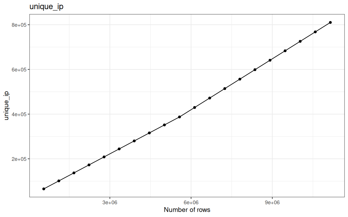
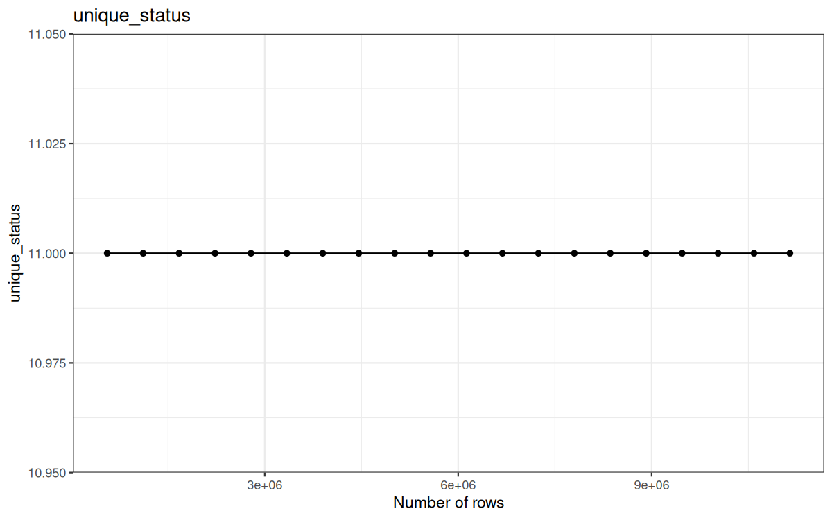
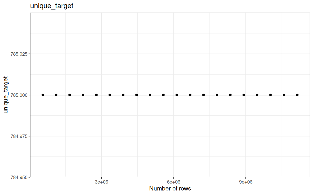
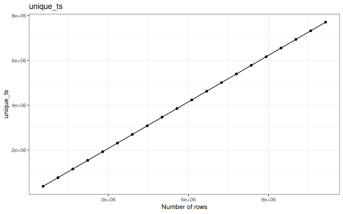
And their cardinality:
library(ggplot2)
library(data.table)
dir.create("describes", showWarnings = FALSE)
plot_df <- data.frame(
log_files = numeric(),
unique_ip = numeric(),
unique_ts = numeric(),
unique_target = numeric(),
unique_status = numeric(),
unique_ua = numeric()
)
for (i in 1:20) {
file_path <- paste0("logs/out", i, ".log")
tb <- data.table::fread(
input = file_path,
sep = "\t",
quote = "\"",
col.names = c("ip", "ts", "target", "status", "ua"),
header = FALSE,
colClasses = list(
character = c(1, 3, 5),
double = 2,
integer = 4
),
showProgress = FALSE
)
cat("\nNEW\n")
print(colnames(tb))
print(paste("nrow:", nrow(tb)))
print(data.table::uniqueN(tb$ip))
print(data.table::uniqueN(tb$ts))
print(data.table::uniqueN(tb$target))
print(data.table::uniqueN(tb$status))
print(data.table::uniqueN(tb$ua))
plot_df <- rbind(
plot_df,
data.frame(
log_files = nrow(tb),
unique_ip = data.table::uniqueN(tb$ip),
unique_ts = data.table::uniqueN(tb$ts),
unique_target = data.table::uniqueN(tb$target),
unique_status = data.table::uniqueN(tb$status),
unique_ua = data.table::uniqueN(tb$ua)
)
)
cat("\n\n")
}
cur_colnames <- setdiff(colnames(plot_df), "log_files")
for (cl in cur_colnames) {
plt <- ggplot(plot_df, aes(x = log_files, y = .data[[cl]])) +
geom_line() +
geom_point() +
labs(
title = cl,
x = "Number of rows",
y = cl
) +
theme_bw()
ggsave(
filename = paste0("describes/", cl, ".png"),
plot = plt,
width = 8,
height = 5,
dpi = 150
)
}
Synthax note:
Because cl is a string, I use the .data pronoun inside ggplot2 to refer to a column programmatically.
.df[[cl]]
Here are the cardinalities plotted on graphs:
Unique ip:
Unique status:
Unique target:
Unique ts:
Unique UA:
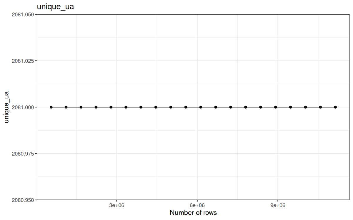
Which is expected, I mean we already stated that the representation of UA, status and target was representatives for my raw 557230 log file...
The benchmarks
A lot of you suggested to use a dedicated package such as bench or microbenchmark.
They are really great to profile operations, they will itere the expression many times and output meaningful results.
bench
Example:
library("bench")
print(bench::mark(
base = mean(1:1000000),
manual = sum(1:1000000) / 1000000,
iterations = 20,
check = TRUE
), width = Inf, n = Inf)
Result:
# A tibble: 2 × 13
expression min median `itr/sec` mem_alloc `gc/sec` n_itr n_gc
<bch:expr> <bch:tm> <bch:tm> <dbl> <bch:byt> <dbl> <int> <dbl>
1 base 5.57ms 5.86ms 172. 23.3KB 0 20 0
2 manual 260.07ns 270.08ns 2852472. 0B 0 20 0
total_time result memory time gc
<bch:tm> <list> <list> <list> <list>
1 116.61ms <dbl [1]> <Rprofmem [9 × 3]> <bench_tm [20]> <tibble [20 × 3]>
2 7.01µs <dbl [1]> <Rprofmem [0 × 3]> <bench_tm [20]> <tibble [20 × 3]>
We can benchmark as many expressions as we want and specify the number of iterations performed for each one.
-
minis the shortest execution time observed across all measured iterations. -
medianis the median execution time and is generally more representative than the minimum because it is less affected by unusually fast or slow runs. -
itr/secis the estimated number of times the expression can be executed per second. -
n_gcis the total number of garbage-collection events recorded during the measured iterations. -
gc/secis the estimated number of garbage-collection events per second. -
mem_allocis the cumulative amount of memory allocated through R’s memory allocator during one benchmark iteration. It is not the peak memory usage, for that we will look at theRSS(cf: the previous article with/usr/bin/time -v ...)
Here we can see that the first expression is not simply an expanded version of the second one.
More specifically, R can optimize sum() when it is applied directly to a compact integer sequence such as 5:10.
Since R 3.5.0, sequences created with expressions such as 1:n can use the ALTREP framework. Instead of immediately storing every integer in memory, R can represent the sequence using metadata such as:
-
its length;
-
its first value;
-
its increment.
Consequently, sum() does not need to traverse or even materialize every value. It has a specialized ALTREP implementation that can directly use the arithmetic-series formula:
n * (first + last) / 2
For example:
6 * (5 + 10) / 2
# [1] 45
This produces the same result as:
sum(5:10)
# [1] 45
Therefore, sum(5:10) can be extremely fast: R already knows that the object represents a regular sequence and computes its sum from the sequence metadata.
By contrast, mean() uses a more general implementation and does not benefit from the specialized ALTREP summation method in the same way. It may therefore have to iterate over the sequence, explaining why it is slower in this particular benchmark.
The small allocation reported for mean(), around 23.3 KB, does not correspond to the mathematical operation itself.
A mean only fundamentally requires an accumulator and a count.
The reported allocation is more likely related to R's evaluation machinery, result creation, method dispatch...
microbenchmark
On a more 'execution time' oriented benchark, we can use microbenchmark.
Example:
library("microbenchmark")
result <- microbenchmark(
base = mean(1:1000000),
manual = sum(1:1000000) / 1000000,
times = 20L,
check = "equal"
)
print(result)
Result:
Unit: nanoseconds
expr min lq mean median uq max neval
base 5523430 5848340 5825735.2 5852485 5854520 5901489 20
manual 230 330 706.5 530 750 3470 20
As you see we see, for each expr:
-
median -
mean -
min -
max -
lq-> low quantile -> Q1 -> It is the value below which approximately 25% of the execution times fall. -
uq-> upper qantile -> Q3 -> It is the value below which approximately 75% of the execution times fall.
Why i won't use them ?
First, the methodology is:
-
20generated log files, from 1× to 20× the original file size. -
6 pipeline variants:
data.tableanddplyr, each withfread,readr, andvroomingestion. -
10 consecutive runs per file and per variant.
-
Execution time measured with
proc.time():elapsed,user,system. -
Memory measured with
gc()counters: current/maxNCellsandVCells. -
Results are interpreted mainly as hot-run behavior, with the first run treated separately as a cold-start signal.
Second, because I want both execution time and memory profiling results.
And also, in R we can make the abstraction of two distinc memory:
For memory, R distinguishes between two main categories in the output of gc():
-
NCells-> Node Cells. They are used for R objects and internal structures such as language objects, pairlists, environments, function calls, symbols, attributes, and the administrative metadata associated with vectors. On a typical 64-bit build of R, one NCell occupies approximately 56 bytes. -
VCells-> Vector Cells. They are primarily used to store the actual contents of vector-like objects, such as integer, double, logical, complex, raw (each element of arawis one byte), character-pointer, list, and expression vectors. OneVCellcorresponds to 8 bytes (64 bits) of vector-heap space.
This distinction can be observed with gc():
Which produces output similar to:
used (Mb) gc trigger (Mb) max used (Mb)
Ncells 350000 18.7 660000 35.3 500000 26.8
Vcells 700000 5.4 8388608 64.0 1200000 9.2
The columns mean:
used-> the amount of memory currently occupied.gc trigger-> the allocation threshold at which R is likely to trigger another garbage-collection cycle.max used-> the highest amount of memory observed since the last reset of the maximum-usage counters.
We reset the max used counters reported by gc() to the current post-GC baseline (see later) by calling gc(reset = TRUE)
The distinction between NCells and VCells can be understood through a vector.
A vector requires both:
-
an R object containing metadata such as its type, length, attributes, and references
-
a memory region containing its actual elements.
The object header and administrative information contribute to NCells, whereas the vector's element storage contributes to VCells.
For example:
gc(reset = TRUE)
x <- numeric(1e6)
gc()
Creates one main vector object (low NCells) but allocates storage for one million double values (pretty high VCells) .
Since a double occupies 8 bytes (1 VCell), the vector payload alone requires approximately:
1,000,000 × 8 bytes = 8 MB
This equals to roughly 1 000 000 VCells.
Look at the results:
used (Mb) gc trigger (Mb) max used (Mb)
Ncells 283017 15.2 664391 35.5 283212 15.2
Vcells 1486332 11.4 8388608 64.0 1486552 11.4
Because gc() measured the VCells and NCells for the whole R process, we do not have exactly 1M VCells but it tends to it.
The approximately 400k VCells in addition and the base NCells we have are due to:
-
base namespaces and loaded base packages
-
symbols and internal tables
-
primitive functions and language objects
-
R’s internal bookkeeping and runtime structures
By contrast, creating many small language objects or list structures increases NCells.
For example:
gc(reset = TRUE)
x <- as.pairlist(rep(1, 1e6))
gc()
Result:
used (Mb) gc trigger (Mb) max used (Mb)
Ncells 2283044 122.0 3525317 188.3 2283082 122
Vcells 1486369 11.4 8388608 64.0 2486385 19
Here we saw that NCells (used) grew from 283017 in the previous example to 2283044 in this one.
VCells barrely changed because in addition we stored the same amount of memory in VCells space.
The distinction can be summarized as:
NCellsrepresent object nodes and administrative structures.VCellsrepresent storage used by vectors.
Because data.table and dplyr use ordinary R vectors to store their values, these measurements are reliable for comparing their memory usage.
Now, for the execution time i won't use Sys.time() since it just gives us the current time.
Hence, a difference such as:
t <- Sys.time()
function_call()
log_step("name of the step", t, df)
With:
log_step <- function(name, start, df = NULL) {
elapsed <- as.numeric(difftime(Sys.time(), start, units = "secs"))
if (!is.null(df)) {
nrows <- nrow(df)
cat(sprintf("[filtered_data] %-25s %.4f sec | rows: %s\n",
name,
elapsed,
format(nrows, big.mark = " ")))
} else {
nrows <- NA_integer_
cat(sprintf("[filtered_data] %-25s %.4f sec\n",
name,
elapsed))
}
bench_data <<- rbind(bench_data, data.frame("seconds" = elapsed,
"nrows" = nrows,
"character" = name
)
)
}
Gives us elapsed time.
This is good enough especialy for only measuring user experienced latency, but we can have more informations.
There are 3 different time indicators:
-
system-> the amount of CPU time spent by the operating-system kernel on behalf of the R process. This includes operations such as reading files, writing files, allocating or mapping memory, managing processes, and performing other system calls. It is sometimes called kernel time. -
user-> the amount of CPU time spent executing code in user space. This includes the time spent running R code and native C, C++, or Fortran code called by R. It does not include time spent inside the operating-system kernel. -
elapsed-> the real wall-clock time between the beginning and the end of the operation. It includes everything that happened during that period: CPU computation, disk or network I/O, waiting for locks, sleeping, scheduling delays, and time spent waiting for other processes or threads. This is generally the best metric for measuring the latency experienced by the user.
Note that if an operation is multithreaded, we can have a higher user time than elapsed time, for example if an operation has an elapsed time of 1.2s and for each thread a user time of 1s and that the operation is multithreaded, then we have a reported user time of 4 * 1s = 4s.
Then, what will i use ?
I will tweak my log_step function I used in the previous article.
For pure execution time.
bench_index <- as.integer(Sys.getenv("BENCH_INDEX", "1"))
bench_data <- data.frame(
elapsed = numeric(),
user = numeric(),
system = numeric(),
nrows = numeric(),
name = character()
)
log_step <- function(name, expr) {
start <- proc.time()
result <- eval.parent(substitute(expr))
delta <- proc.time() - start
elapsed <- delta[["elapsed"]]
user <- delta[["user.self"]]
system <- delta[["sys.self"]]
nrows <- if (!is.null(result) && (is.data.frame(result) || data.table::is.data.table(result))) {
nrow(result)
} else {
NA_integer_
}
bench_data <<- rbind(
bench_data,
data.frame(
elapsed = elapsed,
user = user,
system = system,
nrows = nrows,
name = name
)
)
result
}
speed_dir <- "datatable_results"
all_results_file <- c("1.result",
"2.result",
"3.result",
"4.result",
"5.result",
"6.result",
"7.result",
"8.result",
"9.result",
"10.result",
"11.result",
"12.result",
"13.result",
"14.result",
"15.result",
"16.result",
"17.result",
"18.result",
"19.result",
"20.result"
)
write_benchs <- function() {
write.table(x = bench_data,
file = paste0(speed_dir, "/", all_results_file[bench_index]),
sep = ",",
row.names = FALSE,
col.names = FALSE,
append = TRUE
)
}
The important part here is:
expr-> the expression, still not evaluated, just a promise (lazy)
Now, when it comes to evaluating the expression, I used:
result <- eval.parent(substitute(expr))
Technically, because an R function argument is represented as a promise, it already contains both:
-
the unevaluated expression
-
the environment in which that expression should be evaluated
Furthermore, referring to the argument normally forces the promise. Therefore, in this particular function, I could simply have written:
result <- expr
This would force expr at that exact point and evaluate its stored expression in the environment associated with the promise, which is normally the environment from which log_step() was called.
So why did I use:
result <- eval.parent(substitute(expr))
The main reason is to make the evaluation process explicit.
It can be decomposed into two operations:
-
substitute(expr)-> extracts the unevaluated expression stored in the promise and returns it as an R language object. It does not execute the expression. -
eval.parent()-> evaluates that language object in the parent evaluation frame, which is the environment of the function that calledlog_step()
The complete expression is therefore conceptually equivalent to:
captured_expr <- substitute(expr)
result <- eval(captured_expr, envir = parent.frame())
Using eval.parent(substitute(expr)) introduces a small fixed evaluation overhead compared with directly forcing the promise through result <- expr.
However, the same wrapper is applied to every pipeline implementation, so this overhead is consistent across all variants and does not compromise the relative comparison.
Furthermore, the measured pipeline stages generally take milliseconds or longer, whereas the additional cost of substitute() and eval.parent() is expected to be extremely small in comparison. Its effect on the final measurements is therefore practically negligible.
This overhead would only become important when benchmarking extremely short expressions whose execution time is itself in the microsecond or nanosecond range.
Speaking of baseline cost, we can also include the second proc.time() function call that is also incuded in the benchmark, but also very negligible.
Note that the subsraction from proc.time() - start is not included as a baseline cost because happens just after evaluating proc.time().
This part is for profiling the execution time, but when it comes to profiling memory usage, we tweak it to the following:
bench_index <- as.integer(Sys.getenv("BENCH_INDEX", "1"))
bench_data <- data.frame(
max_ncells_bytes = numeric(),
max_vcells_bytes = numeric(),
current_ncells_bytes = numeric(),
current_vcells_bytes = numeric(),
nrows = numeric(),
name = character()
)
log_step <- function(name, expr) {
gc(reset = TRUE)
result <- eval.parent(substitute(expr))
gc_after <- gc()
nrows <- if (!is.null(result) && (is.data.frame(result) || data.table::is.data.table(result))) {
nrow(result)
} else {
NA_integer_
}
max_ncells_bytes <- gc_after["Ncells", "max used"] * 56
max_vcells_bytes <- gc_after["Vcells", "max used"] * 8
current_ncells_bytes <- gc_after["Ncells", "used"] * 56
current_vcells_bytes <- gc_after["Vcells", "used"] * 8
bench_data <<- rbind(
bench_data,
data.frame(
max_ncells_bytes = data.table::fcoalesce(max_ncells_bytes, -1),
max_vcells_bytes = data.table::fcoalesce(max_vcells_bytes, -1),
current_ncells_bytes = data.table::fcoalesce(current_ncells_bytes, -1),
current_vcells_bytes = data.table::fcoalesce(current_vcells_bytes, -1),
nrows = nrows,
name = name
)
)
result
}
mem_dir <- "datatable_mem_results"
all_results_file <- c("1.result",
"2.result",
"3.result",
"4.result",
"5.result",
"6.result",
"7.result",
"8.result",
"9.result",
"10.result",
"11.result",
"12.result",
"13.result",
"14.result",
"15.result",
"16.result",
"17.result",
"18.result",
"19.result",
"20.result"
)
write_benchs <- function() {
write.table(x = bench_data,
file = paste0(mem_dir, "/", all_results_file[bench_index]),
sep = ",",
row.names = FALSE,
col.names = FALSE,
append = TRUE
)
}
Calling gc(reset = TRUE) before a benchmark run forces a garbage collection cycle and resets the max used counters reported by gc() to the current post-GC heap state.
This means that unreachable R objects can be collected, so the current used values for Vcells and Ncells may decrease before the next measurement.
After that, the max used counters start again from the new post-GC baseline. The following max used values therefore describe the highest absolute heap level reached since that reset, not a pure allocation delta unless we subtract the baseline explicitly.
However, this does not create a fresh R process. Loaded packages, initialized internals, allocator state, symbol tables, string pools, and package-level caches may still remain in memory. Some vectors or internal structures may also be retained or reused by R rather than fully released to the operating system.
For this reason, this benchmark should mainly be interpreted as a hot-run benchmark. My current intuition is that hot-run execution times may be lower because some initialization work has already happened (bacjkend initialization + cached values), while memory usage may remain higher because the R process is not fully fresh between runs.
Even though each log file has only one cold-start outlier, these outliers should not be ignored. They capture a different but important story: the cost of starting from a fresh or less-initialized state, including package initialization, allocator warm-up, internal cache creation, and other one-time setup costs.
I will maybe do another article only measuring cold-start run with more runs for each log-file.
This benchmark is useful for observing the evolution of the whole pipeline, but it is less precise as a strict per-operation memory-allocation benchmark. For that, it would be better to subtract the post-GC baseline explicitly:
gc_before <- gc(reset = TRUE)
pre_current_ncells_bytes <- gc_before["Ncells", "used"] * 56
pre_current_vcells_bytes <- gc_before["Vcells", "used"] * 8
result <- eval.parent(substitute(expr))
gc_after <- gc()
nrows <- if (!is.null(result) && (is.data.frame(result) || data.table::is.data.table(result))) {
nrow(result)
} else {
NA_integer_
}
max_ncells_bytes <- gc_after["Ncells", "max used"] * 56 - pre_current_ncells_bytes
max_vcells_bytes <- gc_after["Vcells", "max used"] * 8 - pre_current_vcells_bytes
current_ncells_bytes <- gc_after["Ncells", "used"] * 56 - pre_current_ncells_bytes
current_vcells_bytes <- gc_after["Vcells", "used"] * 8 - pre_current_vcells_bytes
To get a cleaner per-operation delta from the pre-operation baseline.
That is also someting that I may use in the next article.
Another important part is this:
bench_index <- as.integer(Sys.getenv("BENCH_INDEX", "1"))
Associated with:
all_results_file <- c("1.result",
"2.result",
"3.result",
"4.result",
"5.result",
"6.result",
"7.result",
"8.result",
"9.result",
"10.result",
"11.result",
"12.result",
"13.result",
"14.result",
"15.result",
"16.result",
"17.result",
"18.result",
"19.result",
"20.result"
)
write_benchs <- function() {
write.table(x = bench_data,
file = paste0(speed_dir, "/", all_results_file[bench_index]),
sep = ",",
row.names = FALSE,
col.names = FALSE,
append = TRUE
)
}
Because the whole pipeline will be ran on different log file whose rows will double each time.
For instance later in the benchmark I have:
all_logs_file <- c("logs/out1.log",
"logs/out2.log",
"logs/out3.log",
"logs/out4.log",
"logs/out5.log",
"logs/out6.log",
"logs/out7.log",
"logs/out8.log",
"logs/out9.log",
"logs/out10.log",
"logs/out11.log",
"logs/out12.log",
"logs/out13.log",
"logs/out14.log",
"logs/out15.log",
"logs/out16.log",
"logs/out17.log",
"logs/out18.log",
"logs/out19.log",
"logs/out20.log"
)
file_path <- all_logs_file[bench_index]
And we start the benchmark with this bash script:
#!/usr/bin/env bash
set -e
cp dataset_origin/out1.log logs/out1.log
rm -rf results/datatable_fread_results
mkdir -p results/datatable_fread_results
PORT=7665
URL="http://127.0.0.1:${PORT}"
export BENCH_GLOBAL="speed_global.R"
export BENCH_INGESTION="fread_ing.R"
export BENCH_VARIANT="results/datatable_fread_results"
for i in $(seq 1 20); do
echo
echo "================================"
echo "Running DATA.TABLE - FREAD Speed Benchmark for log file $i"
echo "================================"
profile_dir="$(mktemp -d)"
BENCH_INDEX="$i" Rscript -e "shiny::runApp('.', host='127.0.0.1', port=${PORT}, launch.browser=FALSE)" &
r_pid=$!
echo "Waiting for Shiny server..."
until nc -z 127.0.0.1 "$PORT"; do
sleep 0.2
done
echo "Opening browser..."
firefox \
-no-remote \
-profile "$profile_dir" \
--new-window "$URL" >/dev/null 2>&1 &
firefox_pid=$!
wait "$r_pid"
echo "Shiny stopped for BENCH_INDEX=$i"
kill "$firefox_pid" >/dev/null 2>&1 || true
rm -rf "$profile_dir"
sleep 1
done
echo
echo "All Speed Benchmarks finished."
rm -rf results/datatable_mem_fread_results
mkdir -p results/datatable_mem_fread_results
PORT=7665
URL="http://127.0.0.1:${PORT}"
export BENCH_GLOBAL="mem_global.R"
export BENCH_VARIANT="results/datatable_mem_fread_results"
for i in $(seq 1 20); do
echo
echo "================================"
echo "Running DATA.TABLE - FREAD Mem Benchmark for log file $i"
echo "================================"
profile_dir="$(mktemp -d)"
BENCH_INDEX="$i" Rscript -e "shiny::runApp('.', host='127.0.0.1', port=${PORT}, launch.browser=FALSE)" &
r_pid=$!
echo "Waiting for Shiny server..."
until nc -z 127.0.0.1 "$PORT"; do
sleep 0.2
done
echo "Opening browser..."
firefox \
-no-remote \
-profile "$profile_dir" \
--new-window "$URL" >/dev/null 2>&1 &
firefox_pid=$!
wait "$r_pid"
echo "Shiny stopped for BENCH_INDEX=$i"
kill "$firefox_pid" >/dev/null 2>&1 || true
rm -rf "$profile_dir"
sleep 1
done
echo
echo "All Mem Benchmarks finished."
rm -rf results/datatable_readr_results
mkdir -p results/datatable_readr_results
PORT=7665
URL="http://127.0.0.1:${PORT}"
export BENCH_GLOBAL="speed_global.R"
export BENCH_INGESTION="readr_ing.R"
export BENCH_VARIANT="results/datatable_readr_results"
for i in $(seq 1 20); do
echo
echo "================================"
echo "Running DATA.TABLE - READR Speed Benchmark for log file $i"
echo "================================"
profile_dir="$(mktemp -d)"
BENCH_INDEX="$i" Rscript -e "shiny::runApp('.', host='127.0.0.1', port=${PORT}, launch.browser=FALSE)" &
r_pid=$!
echo "Waiting for Shiny server..."
until nc -z 127.0.0.1 "$PORT"; do
sleep 0.2
done
echo "Opening browser..."
firefox \
-no-remote \
-profile "$profile_dir" \
--new-window "$URL" >/dev/null 2>&1 &
firefox_pid=$!
wait "$r_pid"
echo "Shiny stopped for BENCH_INDEX=$i"
kill "$firefox_pid" >/dev/null 2>&1 || true
rm -rf "$profile_dir"
sleep 1
done
echo
echo "All Speed Benchmarks finished."
rm -rf results/datatable_mem_readr_results
mkdir -p results/datatable_mem_readr_results
PORT=7665
URL="http://127.0.0.1:${PORT}"
export BENCH_GLOBAL="mem_global.R"
export BENCH_VARIANT="results/datatable_mem_readr_results"
for i in $(seq 1 20); do
echo
echo "================================"
echo "Running DATA.TABLE - READR Mem Benchmark for log file $i"
echo "================================"
profile_dir="$(mktemp -d)"
BENCH_INDEX="$i" Rscript -e "shiny::runApp('.', host='127.0.0.1', port=${PORT}, launch.browser=FALSE)" &
r_pid=$!
echo "Waiting for Shiny server..."
until nc -z 127.0.0.1 "$PORT"; do
sleep 0.2
done
echo "Opening browser..."
firefox \
-no-remote \
-profile "$profile_dir" \
--new-window "$URL" >/dev/null 2>&1 &
firefox_pid=$!
wait "$r_pid"
echo "Shiny stopped for BENCH_INDEX=$i"
kill "$firefox_pid" >/dev/null 2>&1 || true
rm -rf "$profile_dir"
sleep 1
done
echo
echo "All Mem Benchmarks finished."
rm -rf results/datatable_vroom_results
mkdir -p results/datatable_vroom_results
PORT=7665
URL="http://127.0.0.1:${PORT}"
export BENCH_GLOBAL="speed_global.R"
export BENCH_INGESTION="vroom_ing.R"
export BENCH_VARIANT="results/datatable_vroom_results"
for i in $(seq 1 20); do
echo
echo "================================"
echo "Running DATA.TABLE - VROOM Speed Benchmark for log file $i"
echo "================================"
profile_dir="$(mktemp -d)"
BENCH_INDEX="$i" Rscript -e "shiny::runApp('.', host='127.0.0.1', port=${PORT}, launch.browser=FALSE)" &
r_pid=$!
echo "Waiting for Shiny server..."
until nc -z 127.0.0.1 "$PORT"; do
sleep 0.2
done
echo "Opening browser..."
firefox \
-no-remote \
-profile "$profile_dir" \
--new-window "$URL" >/dev/null 2>&1 &
firefox_pid=$!
wait "$r_pid"
echo "Shiny stopped for BENCH_INDEX=$i"
kill "$firefox_pid" >/dev/null 2>&1 || true
rm -rf "$profile_dir"
sleep 1
done
echo
echo "All Speed Benchmarks finished."
rm -rf results/datatable_mem_vroom_results
mkdir -p results/datatable_mem_vroom_results
PORT=7665
URL="http://127.0.0.1:${PORT}"
export BENCH_GLOBAL="mem_global.R"
export BENCH_VARIANT="results/datatable_mem_vroom_results"
for i in $(seq 1 20); do
echo
echo "================================"
echo "Running DATA.TABLE - VROOM Mem Benchmark for log file $i"
echo "================================"
profile_dir="$(mktemp -d)"
BENCH_INDEX="$i" Rscript -e "shiny::runApp('.', host='127.0.0.1', port=${PORT}, launch.browser=FALSE)" &
r_pid=$!
echo "Waiting for Shiny server..."
until nc -z 127.0.0.1 "$PORT"; do
sleep 0.2
done
echo "Opening browser..."
firefox \
-no-remote \
-profile "$profile_dir" \
--new-window "$URL" >/dev/null 2>&1 &
firefox_pid=$!
wait "$r_pid"
echo "Shiny stopped for BENCH_INDEX=$i"
kill "$firefox_pid" >/dev/null 2>&1 || true
rm -rf "$profile_dir"
sleep 1
done
echo
echo "All Mem Benchmarks finished."
cd dplyr_variant
bash run_all_bench.sh
The important part is the loop and the environment variable BENCH_INDEX that starts at 1 all the way to 20.
We grab it in global.R to get in what .result file we will store the results:
bench_index <- as.integer(Sys.getenv("BENCH_INDEX", "1"))
...
all_logs_file <- c("logs/out1.log",
"logs/out2.log",
"logs/out3.log",
"logs/out4.log",
"logs/out5.log",
"logs/out6.log",
"logs/out7.log",
"logs/out8.log",
"logs/out9.log",
"logs/out10.log",
"logs/out11.log",
"logs/out12.log",
"logs/out13.log",
"logs/out14.log",
"logs/out15.log",
"logs/out16.log",
"logs/out17.log",
"logs/out18.log",
"logs/out19.log",
"logs/out20.log"
)
file_path <- all_logs_file[bench_index]
Also:
-
set -e-> if a comand returns a non-zero exit status (apart from condition environment), then the script is exited -
until nc -z 127.0.0.1 "$PORT"; do sleep 0.2; done-> test if the connection at127.0.0.1:7665is accepted, if no sleep during 200ms and retry -
wait "$r_pid"-> sleep until the R process ends
Now, what about the temporary "$profile_dir" ?
Firefox uses a folder for each session that is used for:
-
cache
-
cookies
-
local storage
-
session data
-
extensions
-
preferences
-
previously opened tabs
-
Shiny client-side state
So a fresh session for each new benchmark on a new log file.
rm -rf datatable_results
mkdir -p datatable_results
#rm -rf datatable_mem_results
#mkdir -p datatable_mem_results
For the same ingestion backend, we first measure execution time and then memory usage thanks to BENCH_GLOBAL:
source(Sys.getenv("BENCH_GLOBAL", "speed_global.R"))
Then we whange the ingestion backend thanks to BENCH_INGESTION:
source(Sys.getenv("BENCH_INGESTION", "fread_ing.R"))
We have the same for the dplyr variant.
And for each pass, we iterate 10 consecutives time.
Look at what we have in ui.R:
tags$script(HTML("
Shiny.addCustomMessageHandler('reload_app', function(message) {
const key = 'shiny_bench_reload_count';
const maxReloads = 9;
const delay = 500;
let count = parseInt(localStorage.getItem(key) || '0', 10);
if (count < maxReloads) {
localStorage.setItem(key, count + 1);
setTimeout(function() {
window.location.reload();
}, delay);
} else {
localStorage.removeItem(key);
console.log('Benchmark reload loop finished');
Shiny.setInputValue('bench_finished', Math.random(), {priority: 'event'});
}
});
"))
This function acts as a message receiver for he most part and only as a sender for telling the server to stop when the 10 consecutives run are done here:
// Cleaning process
localStorage.removeItem(key);
console.log('Benchmark reload loop finished');
// Sends message
Shiny.setInputValue('bench_finished', Math.random(), {priority: 'event'});
The rest of the time it:
-
Sends a request to reload the page to te browser with the configured delay, letting time for the server or UI to finish potentialy remainding operations
-
Waits for a message from the server named reload_app
-
Defines the key shiny_bench_reload_count, which is used to store the reload counter in
localStorage. On the first pass, this entry does not exist yet, solocalStorage.getItem()returns null. This is handled by the fallback value used later. -
Reads the configuration values.
-
let count = parseInt(localStorage.getItem(key) || '0', 10);retrieves the current value stored under the key. If the entry does not exist, it falls back to the string'0', which is then parsed as a base-10 integer. -
localStorage.setItem(key, count + 1);creates or updates thelocalStorageentry with the incremented reload count. -
Schedules a page reload after the configured delay. This gives client-side or server-side operations a short amount of time to finish before the page is reloaded (normally they are already finished but just to be sure)
And in server.R:
output$kpi_med_readtime <- renderText({
df <- filtered_data()
log_step("KPI MEDIAN READTIME", {
req(nrow(df) > 0)
keep <- !is.na(df$time_on_page) &
df$time_on_page > 0 &
df$time_on_page < 3600
median_time <- df[keep, median(time_on_page)]
if (is.na(median_time)) return("—")
mins <- floor(median_time / 60)
secs <- round(median_time %% 60)
})
result <- sprintf("%02d:%02d", mins, secs)
session$onFlushed(function() { # Here we send he message
session$sendCustomMessage("reload_app", list())
}, once = TRUE)
result
})
It is here that we expect the reload message 'reload_app' to be sent, because it is the last pipeline step.
observeEvent(input$bench_finished, {
write_benchs()
shiny::stopApp()
})
Still in server.R we just listen to the stop-server message, if we receive it we write the benchmark values to the current iteration file.
We do the exact same thing for the dplyr variant.
Note: All measured operations must be disjoint.
For example, inside load_raw_data <- function(file_path), i have several operations measured.
Hence, in server.R (where this function is called), I can not do the following:
log_step("Read First", {
raw_data <- load_raw_data(file_path)
})
It would false the results.
Analysis
Once I get the results in the folders, I can run a R script to plot the results as box-plots.
Those box-plot graphs (named type 1 graphs) will be per operation:
-
x-axis-> the initial rows in the dataframe -
y-axis-> the execution time (user, system, elapsed) or memory consumption ( max/currentNCells,VCells) -
color-> the current rows in the dataframe for the related operation
We will also output boxplots summing the elapsed time for all data manipulation functions per log-file.
That's the type 2 graph.
For each metric, we will also output box-plots per unique log-file per operation (in order).
That's the type 3 graph.
But remember, at this point I have my benchmark results in those folders:
❯ tree results
results
├── datatable_fread_results
│ ├── 10.result
│ ├── 11.result
│ ├── 12.result
│ ├── 13.result
│ ├── 14.result
│ ├── 15.result
│ ├── 16.result
│ ├── 17.result
│ ├── 18.result
│ ├── 19.result
│ ├── 1.result
│ ├── 20.result
│ ├── 2.result
│ ├── 3.result
│ ├── 4.result
│ ├── 5.result
│ ├── 6.result
│ ├── 7.result
│ ├── 8.result
│ └── 9.result
├── datatable_mem_fread_results
│ ├── 10.result
│ ├── 11.result
│ ├── 12.result
│ ├── 13.result
│ ├── 14.result
│ ├── 15.result
│ ├── 16.result
│ ├── 17.result
│ ├── 18.result
│ ├── 19.result
│ ├── 1.result
│ ├── 20.result
│ ├── 2.result
│ ├── 3.result
│ ├── 4.result
│ ├── 5.result
│ ├── 6.result
│ ├── 7.result
│ ├── 8.result
│ └── 9.result
├── datatable_mem_readr_results
│ ├── 10.result
│ ├── 11.result
│ ├── 12.result
│ ├── 13.result
│ ├── 14.result
│ ├── 15.result
│ ├── 16.result
│ ├── 17.result
│ ├── 18.result
│ ├── 19.result
│ ├── 1.result
│ ├── 20.result
│ ├── 2.result
│ ├── 3.result
│ ├── 4.result
│ ├── 5.result
│ ├── 6.result
│ ├── 7.result
│ ├── 8.result
│ └── 9.result
...
And in each file results are formated as:
for execution time:
1.361,1.24,0.095,1114460,"RAW Ingestion"
0.024,0.016,0.00900000000000001,1114460,"Date mutation"
0,0,0,1114460,"Selection"
0.186,0.209,0.037,980880,"Filtering"
0.000999999999999446,0,0,980880,"Status Drop"
0.0139999999999993,0.0130000000000003,0.001,21078,"Time Window"
0.0209999999999999,0.0460000000000003,0.001,NA,"UA Agent Pre"
0,0.00099999999999989,0,11035,"UA Agent"
0.00499999999999989,0.0289999999999999,0,7717,"Asset heuristic"
0.00300000000000011,0.0150000000000001,0,1636,"Article filtering"
0.00300000000000011,0.00500000000000034,0,454,"Rate heuristic"
0.00199999999999978,0.00599999999999978,0,192,"Read time heuristic"
0.00600000000000023,0.0220000000000002,0,192,"ASN Enrichment"
0.00300000000000011,0.0150000000000001,0,192,"ASN Filtering 1"
0.00199999999999978,0.00099999999999989,0,192,"ASN Filtering 2"
0.00100000000000033,0,0,192,"IP Exclusion"
0,0.00099999999999989,0,188,"HONEY POTS"
0,0.00099999999999989,0,NA,"KPI MEDIAN READTIME"
0.673,1.313,0.06,1114460,"RAW Ingestion"
0.0119999999999996,0.000999999999999446,0.01,1114460,"Date mutation"
0,0,0,1114460,"Selection"
0.194999999999999,0.242,0.005,980880,"Filtering"
0,0,0,980880,"Status Drop"
0.00299999999999923,0.00399999999999956,0.001,21078,"Time Window"
0.0220000000000002,0.0440000000000005,0,NA,"UA Agent Pre"
0,0,0,11035,"UA Agent"
0.00600000000000023,0.0289999999999999,0,7717,"Asset heuristic"
0.00299999999999923,0.0169999999999995,0,1636,"Article filtering"
0.00200000000000067,0.00300000000000011,0,454,"Rate heuristic"
0.00199999999999978,0.00299999999999923,0,192,"Read time heuristic"
0.0140000000000002,0.0250000000000004,0,192,"ASN Enrichment"
0.00299999999999923,0.0209999999999999,0,192,"ASN Filtering 1"
0.00100000000000033,0.00199999999999978,0,192,"ASN Filtering 2"
0,0,0,192,"IP Exclusion"
0.00100000000000033,0,0,188,"HONEY POTS"
0,0,0,NA,"KPI MEDIAN READTIME"
... 8 more times
And for memory usage:
149886576,108651952,109109672,68450952,1114460,"RAW Ingestion"
110964224,97467832,110636736,77880176,1114460,"Date mutation"
110680528,77919368,110658072,77888216,1114460,"Selection"
110877088,131057704,110659472,72008784,980880,"Filtering"
110790120,72046568,110659696,68085328,980880,"Status Drop"
112237384,77222456,112078288,69251472,21078,"Time Window"
112092400,70231160,112078960,69519984,NA,"UA Agent Pre"
112127120,70196112,112078960,69118264,11035,"UA Agent"
112249200,69923248,112080080,68778576,7717,"Asset heuristic"
112130760,68930272,112079912,68522024,1636,"Article filtering"
112903504,68984344,112202496,68516024,454,"Rate heuristic"
112982520,68970672,112332752,68522200,192,"Read time heuristic"
113411200,69675480,112613088,68643240,192,"ASN Enrichment"
114105600,69037416,112632856,68650264,192,"ASN Filtering 1"
113337392,68882528,112632128,68649304,192,"ASN Filtering 2"
112681744,68681600,112630560,68648872,192,"IP Exclusion"
112796320,68708152,112630896,68648808,188,"HONEY POTS"
112863520,68707792,112709800,68643528,NA,"KPI MEDIAN READTIME"
121459464,152055848,121117752,111933944,1114460,"RAW Ingestion"
121341192,138725952,121117920,120849704,1114460,"Date mutation"
121136288,120851280,121118088,120849784,1114460,"Selection"
121206960,216988160,121000880,114928752,980880,"Filtering"
121131528,114966576,121001104,111005336,980880,"Status Drop"
121575328,119819472,121424408,111883400,21078,"Time Window"
121438352,112863128,121424912,112151952,NA,"UA Agent Pre"
121473072,112828120,121424912,111750272,11035,"UA Agent"
121593584,112552480,121425080,111410008,7717,"Asset heuristic"
121475760,111561744,121424912,111153496,1636,"Article filtering"
122081960,111384688,121426032,111106536,454,"Rate heuristic"
122050656,111335400,121426760,111068752,192,"Read time heuristic"
128465736,112031456,121434768,111097392,192,"ASN Enrichment"
122906784,111458912,121435944,111097496,192,"ASN Filtering 1"
122140480,111329808,121435216,111096584,192,"ASN Filtering 2"
121484776,111128920,121433592,111096192,192,"IP Exclusion"
121599296,111155416,121433872,111096072,188,"HONEY POTS"
121570624,111086496,121421720,111058696,NA,"KPI MEDIAN READTIME"
121503760,152077224,121128728,111942552,1114460,"RAW Ingestion"
... 8 more times
So this is:
-
metrics in column
-
consecutive operations for the same run in row.
To get the results of a run in a distinct container we need to perform a rotation.
Because this is a rotating patttern we can simply do:
data <- read.table(speed_file,
sep = ",",
header = FALSE
)
elapsed <- as.data.frame(matrix(data$V1,
ncol = length(label),
byrow=TRUE
)
)
... and so on
This constructs a matrix with the consecutive length(label) = 19 cells values on the same rows until the end of the vector, then we convert it to a data.frame so we have one operation per column and 10 rows. A row corresponds to a run.
We do that for each metric (choosing the right column/vector from data)
At this point, we have already created lists of data.frame, one for each metric:
In the same time we create a simple list of 20 data.frame(s) that will serve for plotting the type 2 graphic.
elapsed_line <- vector("list", length(label))
system_line <- vector("list", length(label))
user_line <- vector("list", length(label))
max_ncells_line <- vector("list", length(label))
max_vcells_line <- vector("list", length(label))
current_ncells_line <- vector("list", length(label))
current_vcells_line <- vector("list", length(label))
tot_lines <- vector("list", nb_iter)
for (i in 1:length(label)) {
elapsed_line[[i]] <- data.frame("nrows" = numeric(),
"nrows_df" = numeric(),
"val" = numeric()
)
system_line[[i]] <- data.frame("nrows" = numeric(),
"nrows_df" = numeric(),
"val" = numeric()
)
user_line[[i]] <- data.frame("nrows" = numeric(),
"nrows_df" = numeric(),
"val" = numeric()
)
max_ncells_line[[i]] <- data.frame("nrows" = numeric(),
"nrows_df" = numeric(),
"val" = numeric()
)
max_vcells_line[[i]] <- data.frame("nrows" = numeric(),
"nrows_df" = numeric(),
"val" = numeric()
)
current_ncells_line[[i]] <- data.frame("nrows" = numeric(),
"nrows_df" = numeric(),
"val" = numeric()
)
current_vcells_line[[i]] <- data.frame("nrows" = numeric(),
"nrows_df" = numeric(),
"val" = numeric()
)
}
Their length is the number of operations (length(label)).
Then, we iterate on each of the results file, create the well-formated data.frame (one column for each operation) for memory consumption and execution time results and for each operations metrics we append the new results.
We also create a column associating the current rows the operation is performed on (nrows) and the original log rows number (nrows_df) allowing to identify the run later in the plot function.
tot_lines data.frame(s) will just be one-row dataframe containing the current nrows_df and the elapsed-time sum of all datamanipulation operations.
tot_lines[[I]] <- data.frame("nrows_df" = numeric(),
"val" = numeric()
)
...
tot_vals <-rowSums(elapsed[, 1:length(label)])
tot_lines[[I]] <- rbind(tot_lines[[I]],
data.frame("nrows_df" = rep(rows_log, cur_iter),
"val" = tot_vals
)
)
Here is the whole part.
for (I in 1:nb_iter) {
tot_lines[[I]] <- data.frame("nrows_df" = numeric(),
"val" = numeric()
)
speed_file <- paste0(speed_folder, "/", I, ".result")
mem_file <- paste0(mem_folder, "/", I, ".result")
data <- read.table(speed_file,
sep = ",",
header = FALSE
)
elapsed <- as.data.frame(matrix(data$V1,
ncol = length(label),
byrow=TRUE
)
)
cur_iter <- nrow(elapsed)
user <- as.data.frame(matrix(data$V2,
ncol = length(label),
byrow=TRUE
)
)
system <- as.data.frame(matrix(data$V3,
ncol = length(label),
byrow=TRUE
)
)
n_rows <- as.data.frame(matrix(data$V4,
ncol = length(label),
byrow=TRUE
)
)
n_rows$V1 = data.table::shift(n_rows$V1,
type="lag",
fill=count_lines(paste0("logs/out", I, ".log"))
)
data <- read.table(mem_file,
sep = ",",
header = FALSE
)
max_ncells <- as.data.frame(matrix(data$V1,
ncol = length(label),
byrow=TRUE
)
)
max_vcells <- as.data.frame(matrix(data$V2,
ncol = length(label),
byrow=TRUE
)
)
current_ncells <- as.data.frame(matrix(data$V3,
ncol = length(label),
byrow=TRUE
)
)
current_vcells <- as.data.frame(matrix(data$V4,
ncol = length(label),
byrow=TRUE
)
)
rows_log <- n_rows[1, 1]
for (i in 1:length(label)) {
elapsed_line[[i]] <- rbind(elapsed_line[[i]],
data.frame("nrows" = rep(n_rows[1, i], cur_iter),
"nrows_df" = rep(rows_log, cur_iter),
"val" = elapsed[, i]
)
)
user_line[[i]] <- rbind(user_line[[i]],
data.frame("nrows" = rep(n_rows[1, i], cur_iter),
"nrows_df" = rep(rows_log, cur_iter),
"val" = user[, i]
)
)
system_line[[i]] <- rbind(system_line[[i]],
data.frame("nrows" = rep(n_rows[1, i], cur_iter),
"nrows_df" = rep(rows_log, cur_iter),
"val" = system[, i]
)
)
max_ncells_line[[i]] <- rbind(max_ncells_line[[i]],
data.frame("nrows" = rep(n_rows[1, i], cur_iter),
"nrows_df" = rep(rows_log, cur_iter),
"val" = max_ncells[, i]
)
)
max_vcells_line[[i]] <- rbind(max_vcells_line[[i]],
data.frame("nrows" = rep(n_rows[1, i], cur_iter),
"nrows_df" = rep(rows_log, cur_iter),
"val" = max_vcells[, i]
)
)
current_ncells_line[[i]] <- rbind(current_ncells_line[[i]],
data.frame("nrows" = rep(n_rows[1, i], cur_iter),
"nrows_df" = rep(rows_log, cur_iter),
"val" = current_ncells[, i]
)
)
current_vcells_line[[i]] <- rbind(current_vcells_line[[i]],
data.frame("nrows" = rep(n_rows[1, i], cur_iter),
"nrows_df" = rep(rows_log, cur_iter),
"val" = current_vcells[, i]
)
)
cat(paste("\n", label[i], "\n"))
}
tot_vals <-rowSums(elapsed[, 1:length(label)])
tot_lines[[I]] <- rbind(tot_lines[[I]],
data.frame("nrows_df" = rep(rows_log, cur_iter),
"val" = tot_vals
)
)
cat(paste("\n\n", rows_log, "\n\n"))
}
Now, for the type 3 graphs we need to have a data.frame for each metric containing results per operations per nrows_df
We can just rbind() all data.frame(s) per metric.
Each time we append a data.frame to the final one for the current metric, we add the results of the runs for the next operation, so we also need to addd an operation column to identify them:
First we create a data.frame list by metric type:
overlay_time_df <- vector("list", 3)
names(overlay_time_df) <- c("user",
"system",
"elapsed")
overlay_memory_df <- vector("list", 4)
names(overlay_memory_df) <- c("current_ncells",
"current_vcells",
"max_ncells",
"max_vcells")
for (i in 1:length(overlay_time_df)) {
overlay_time_df[[i]] <- data.frame("nrows" = numeric(),
"nrows_df" = numeric(),
"val" = numeric(),
"operation" = character()
)
}
for (i in 1:length(overlay_memory_df)) {
overlay_memory_df[[i]] <- data.frame("nrows" = numeric(),
"nrows_df" = numeric(),
"val" = numeric(),
"operation" = character()
)
}
Then we do what we spoke about:
for (i in 1:length(label)) {
cur_op <- label[i]
overlay_time_df$user <- rbind(overlay_time_df$user,
cbind(user_line[[i]], operation = rep(cur_op, global_iter))
)
overlay_time_df$system <- rbind(overlay_time_df$system,
cbind(system_line[[i]], operation = rep(cur_op, global_iter))
)
overlay_time_df$elapsed <- rbind(overlay_time_df$elapsed,
cbind(elapsed_line[[i]], operation = rep(cur_op, global_iter))
)
overlay_memory_df$current_ncells <- rbind(overlay_memory_df$current_ncells,
cbind(current_ncells_line[[i]], operation = rep(cur_op, global_iter))
)
overlay_memory_df$current_vcells <- rbind(overlay_memory_df$current_vcells,
cbind(current_vcells_line[[i]], operation = rep(cur_op, global_iter))
)
overlay_memory_df$max_ncells <- rbind(overlay_memory_df$max_ncells,
cbind(max_ncells_line[[i]], operation = rep(cur_op, global_iter))
)
overlay_memory_df$max_vcells <- rbind(overlay_memory_df$max_vcells,
cbind(max_vcells_line[[i]], operation = rep(cur_op, global_iter))
)
}
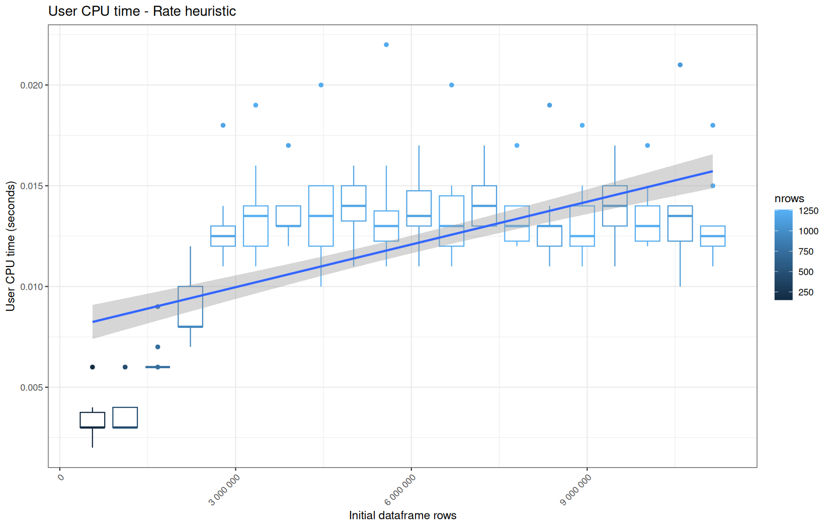
Finally here is the type 1 graph function:
draw_boxplot <- function(df, title, ylab, outfile) {
if (is.null(df) || nrow(df) == 0) {
message("Skipping empty plot: ", title)
return(invisible(NULL))
}
p <- ggplot(df, aes(x = nrows_df, y = val, color = nrows)) +
geom_boxplot(aes(group = nrows_df)) +
geom_smooth(
method = "lm",
se = TRUE,
level = 0.95
) +
labs(
title = title,
x = "Initial dataframe rows",
y = ylab
) +
scale_x_continuous(
labels = function(x) format(x, big.mark = " ", scientific = FALSE)
) +
theme_bw() +
theme(
axis.text.x = element_text(angle = 45, hjust = 1)
)
ggsave(
filename = outfile,
plot = p,
width = 11,
height = 7,
dpi = 150
)
}
Used on both metrics type:
for (i in seq_along(label)) {
step_name <- label[i]
file_name <- safe_name(step_name)
draw_boxplot(
elapsed_line[[i]],
paste("Elapsed time -", step_name),
"Elapsed time (seconds)",
file.path(out_plot, paste0("elapsed_", file_name, ".png"))
)
draw_boxplot(
user_line[[i]],
paste("User CPU time -", step_name),
"User CPU time (seconds)",
file.path(out_plot, paste0("user_", file_name, ".png"))
)
draw_boxplot(
system_line[[i]],
paste("System CPU time -", step_name),
"System CPU time (seconds)",
file.path(out_plot, paste0("system_", file_name, ".png"))
)
}
for (i in seq_along(label)) {
step_name <- label[i]
file_name <- safe_name(step_name)
draw_boxplot(
max_ncells_line[[i]],
paste("Max Ncells -", step_name),
"Max Ncells bytes",
file.path(out_plot_mem, paste0("max_ncells_", file_name, ".png"))
)
draw_boxplot(
max_vcells_line[[i]],
paste("Max Vcells -", step_name),
"Max Vcells bytes",
file.path(out_plot_mem, paste0("max_vcells_", file_name, ".png"))
)
draw_boxplot(
current_ncells_line[[i]],
paste("Current Ncells -", step_name),
"Current Ncells bytes",
file.path(out_plot_mem, paste0("current_ncells_", file_name, ".png"))
)
draw_boxplot(
current_vcells_line[[i]],
paste("Current Vcells -", step_name),
"Current Vcells bytes",
file.path(out_plot_mem, paste0("current_vcells_", file_name, ".png"))
)
}
Example:
Now, the type 2 graph:
draw_total_boxplot <- function(df, title, ylab, outfile) {
p <- ggplot(df, aes(x = nrows_df, y = val)) +
geom_boxplot(aes(group = nrows_df)) +
geom_smooth(
method="lm",
se = TRUE,
level = 0.85
) +
labs(
title = title,
x = "Initial dataframe rows",
y = ylab
) +
theme_bw() +
theme(
axis.text.x = element_text(angle = 45, hjust = 1)
)
ggsave(
filename = outfile,
plot = p,
width = 11,
height = 7,
dpi = 150
)
}
Because this one represent log-files on the x-axis, we must fold a rbind on the list containing the total elapsed time data.frame(s):
tot_df <- do.call(rbind, tot_lines)
draw_total_boxplot(
tot_df,
"Total pipeline elapsed time",
"Total elapsed time (seconds)",
file.path(out_plot, "total_pipeline_elapsed.png")
)
Example:

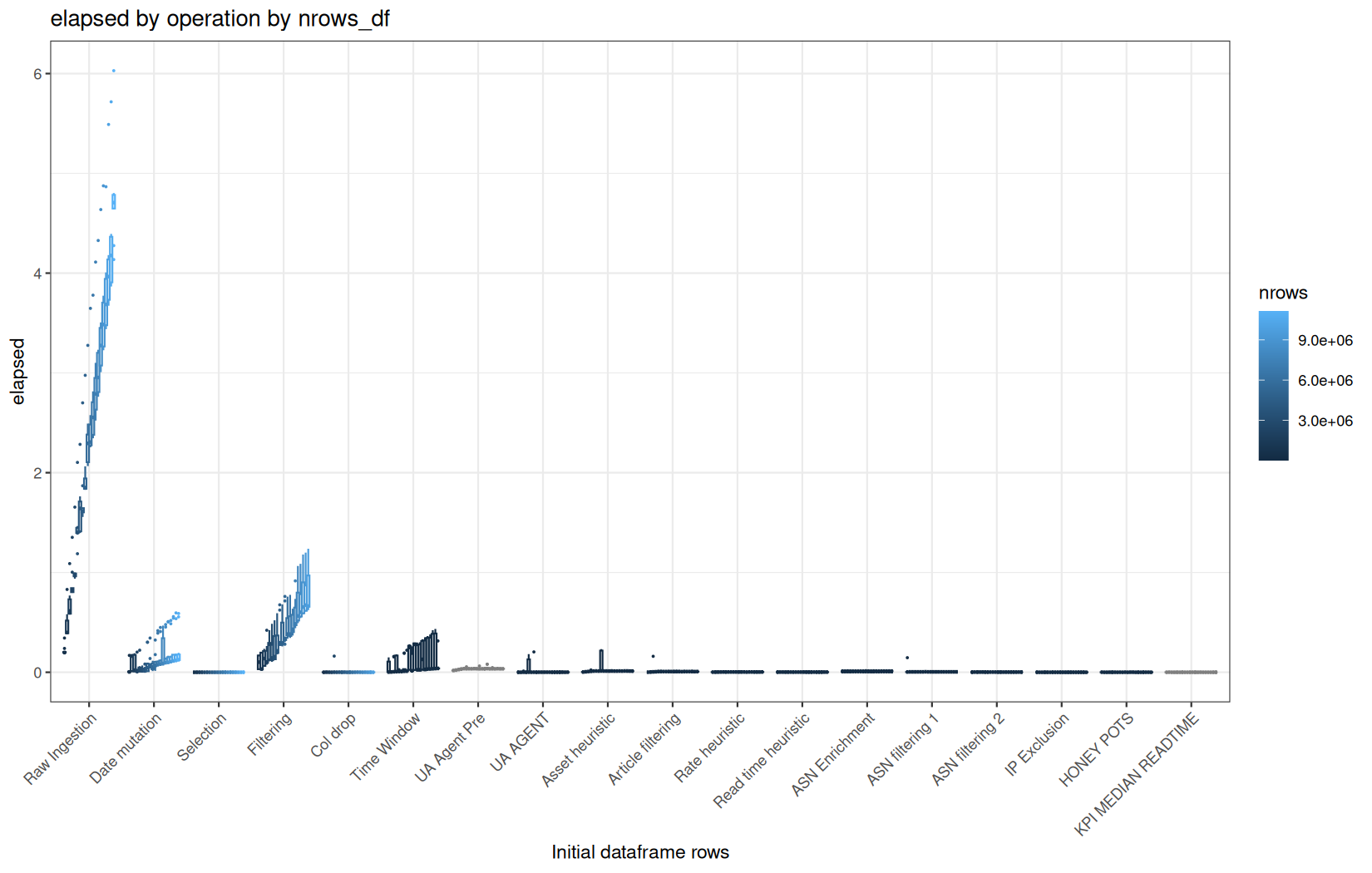
Finally, for the type 3 graph.
Because we'll use interaction(operations, nrows_df), we also need to make nrows_df a factor which levels will be of course ascendly sorted.
And we make sure the operations are also sorted in the right order (label order).
draw_boxplot_operations <- function(df, title, ylab, outfile) {
df$operation <- factor(df$operation, levels = label)
df$nrows_df <- factor(df$nrows_df, levels = sort(unique(df$nrows_df)))
p <- ggplot(df, aes(x = operation, y = val, color = nrows)) +
geom_boxplot(aes(group = interaction(operation, nrows_df)),
position = position_dodge(width = 0.8),
outlier.size = 0.2
) +
labs(
title = title,
x = "Initial dataframe rows",
y = ylab
) +
theme_bw() +
theme(
axis.text.x = element_text(angle = 45, hjust = 1)
)
ggsave(
filename = outfile,
plot = p,
width = 11,
height = 7,
dpi = 150
)
}
And we just apply them:
for (i in 1:length(overlay_time_df)) {
cur_metric <- names(overlay_time_df)[i]
draw_boxplot_operations(overlay_time_df[[i]],
paste(cur_metric, "by operation by nrows_df"),
cur_metric,
file.path(out_plot, paste0(cur_metric, "_metric.png"))
)
}
for (i in 1:length(overlay_memory_df)) {
cur_metric <- names(overlay_memory_df)[i]
draw_boxplot_operations(overlay_memory_df[[i]],
paste(cur_metric, "by operation by nrows_df"),
cur_metric,
file.path(out_plot, paste0(cur_metric, "_metric.png"))
)
}
Example:
The Results
Ingestion
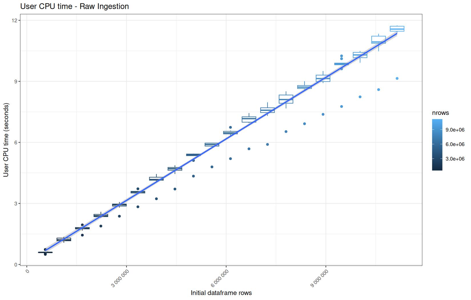
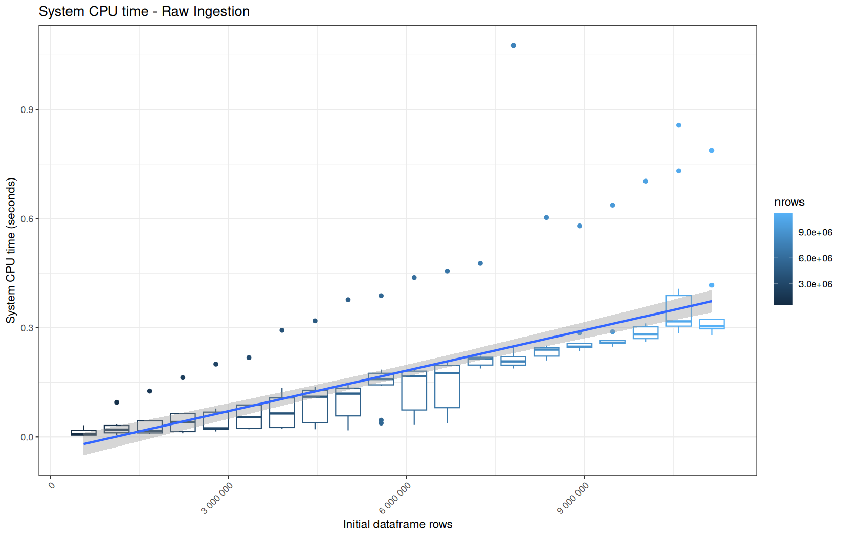
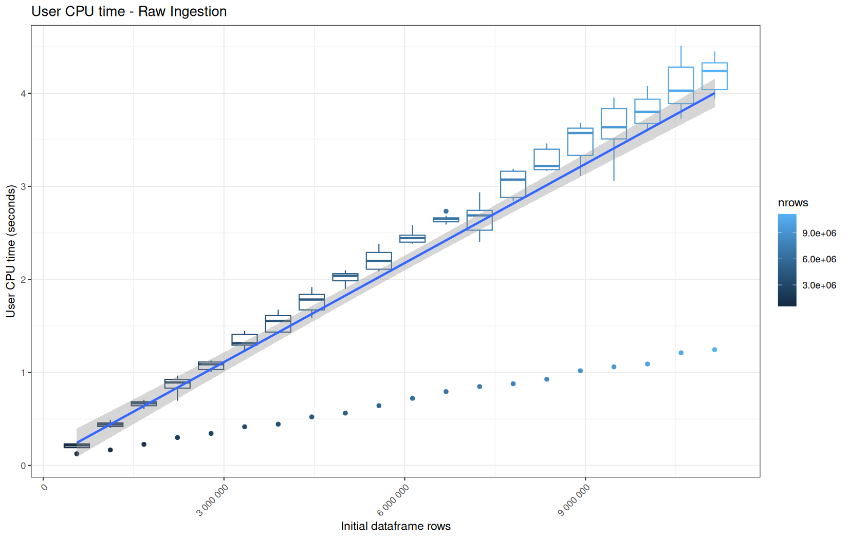
Execution Time
data.table
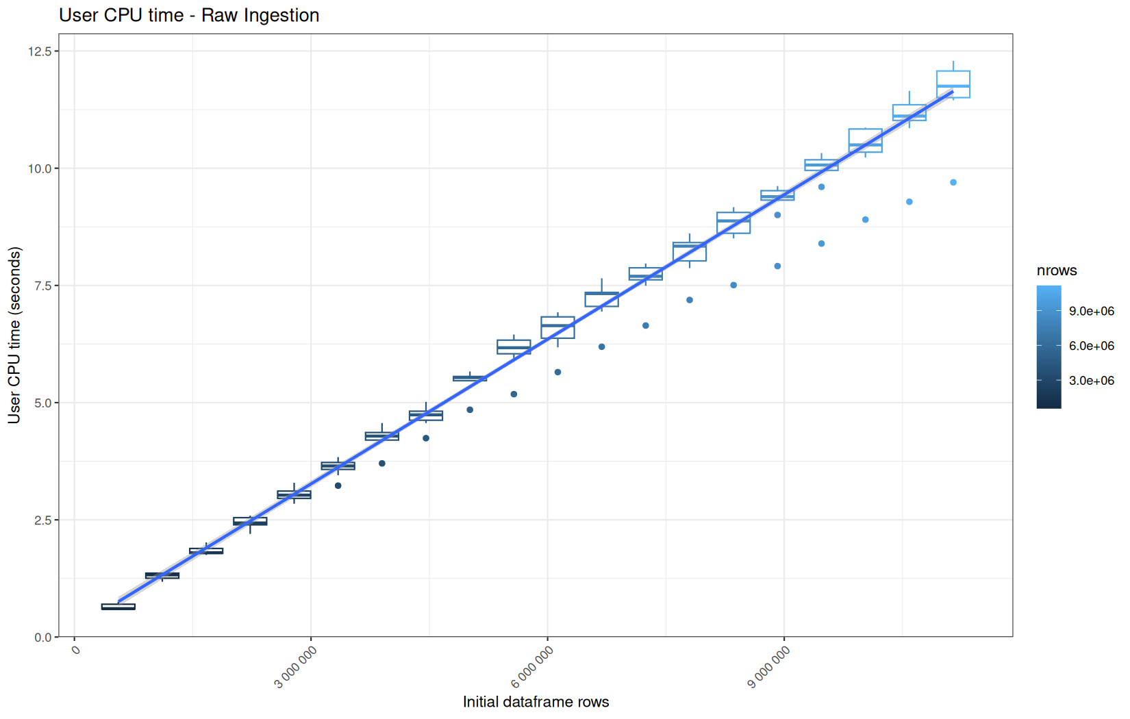
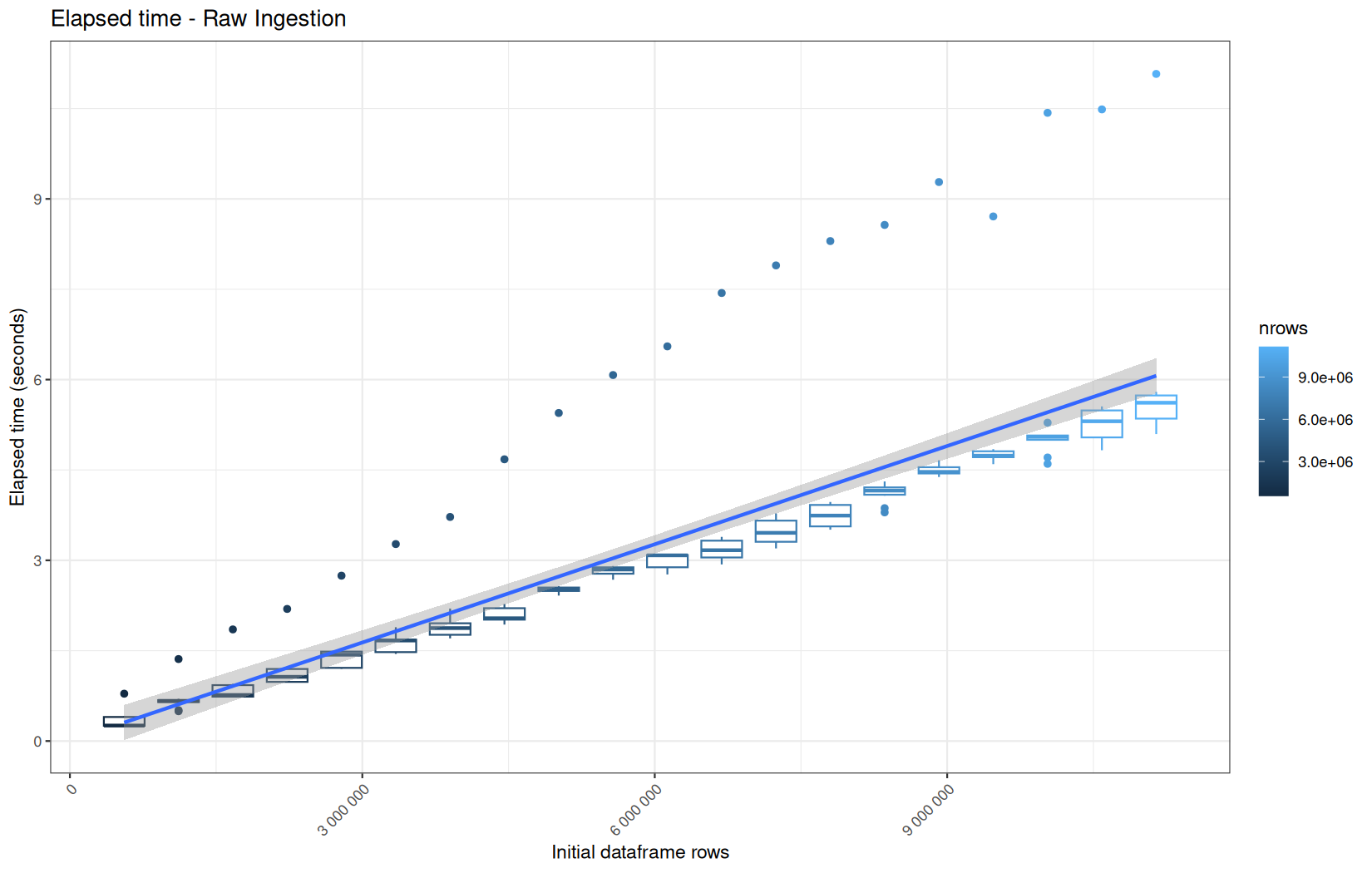
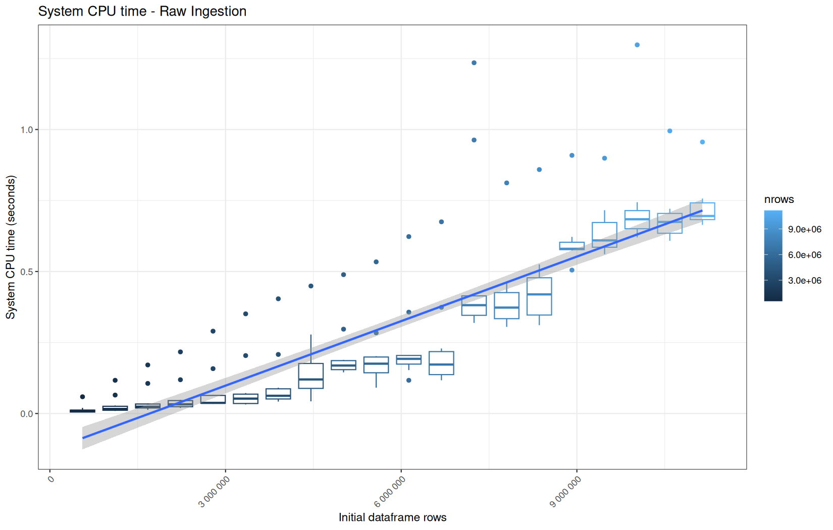
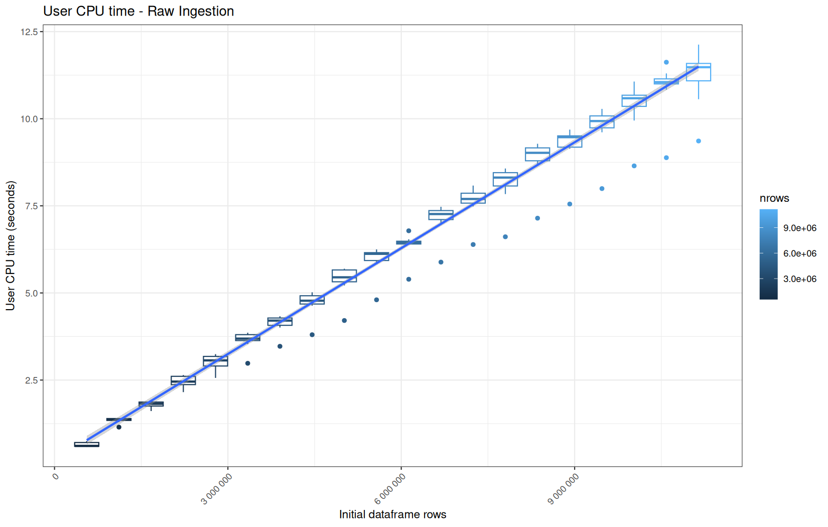
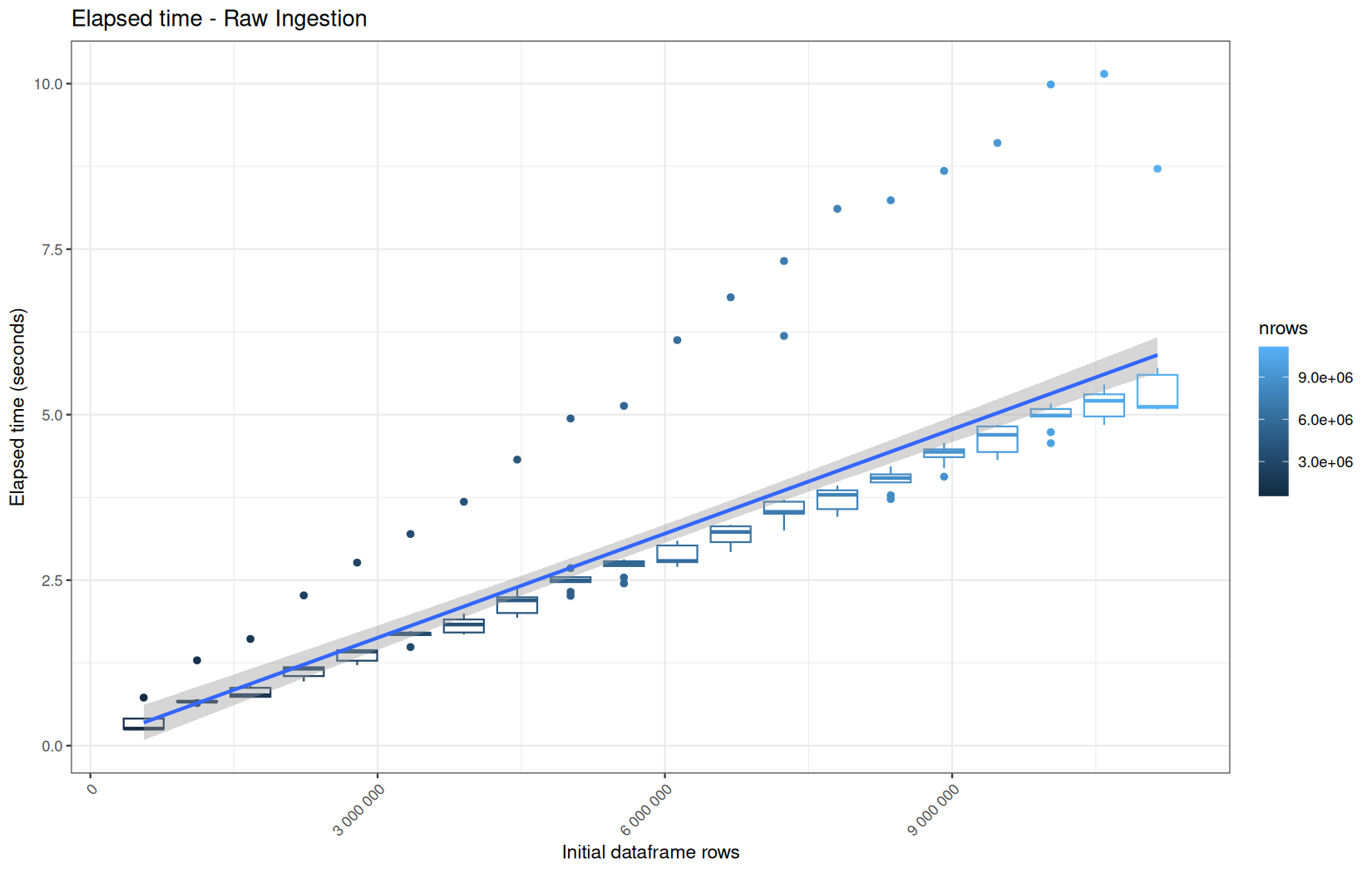
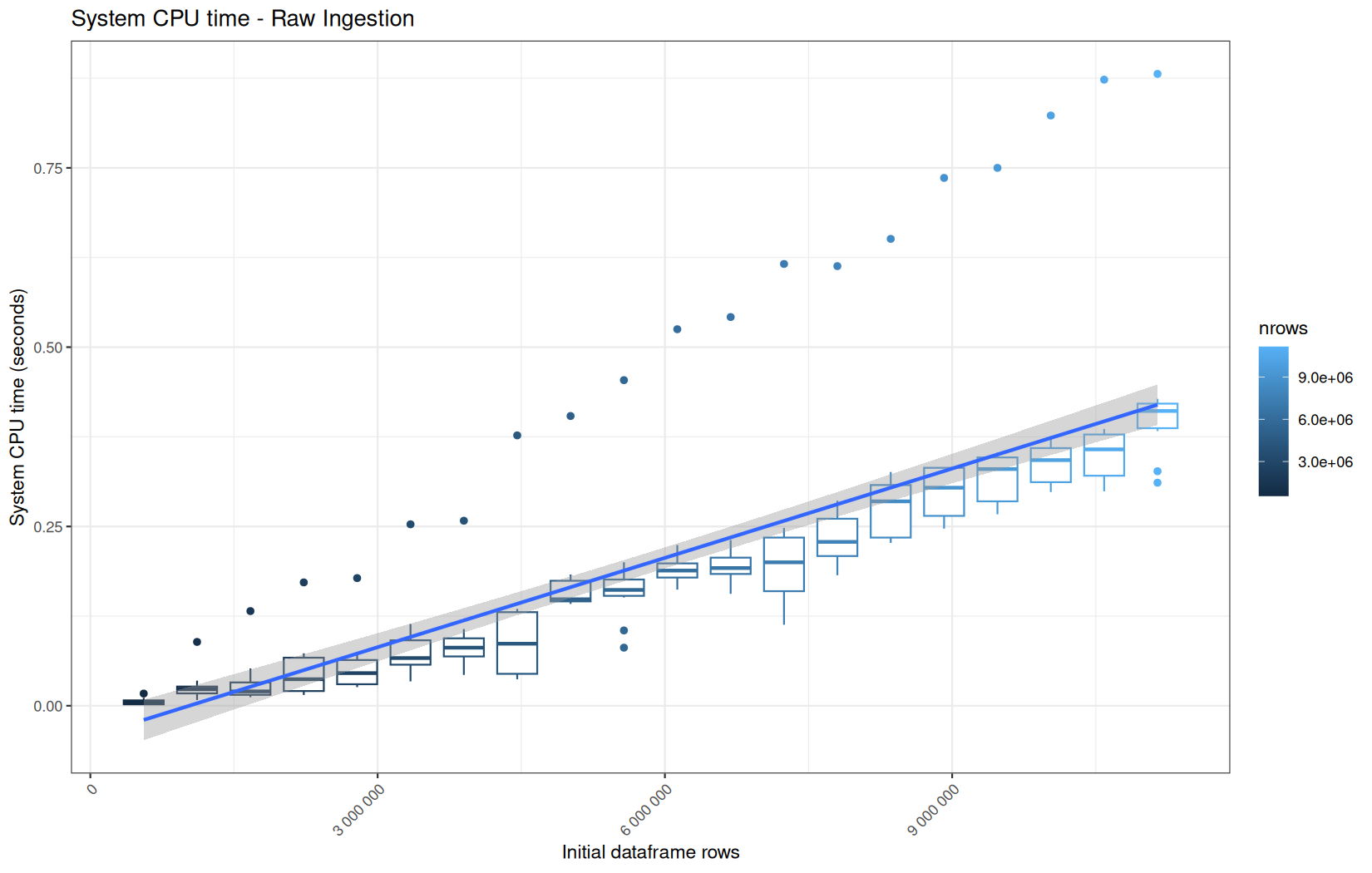
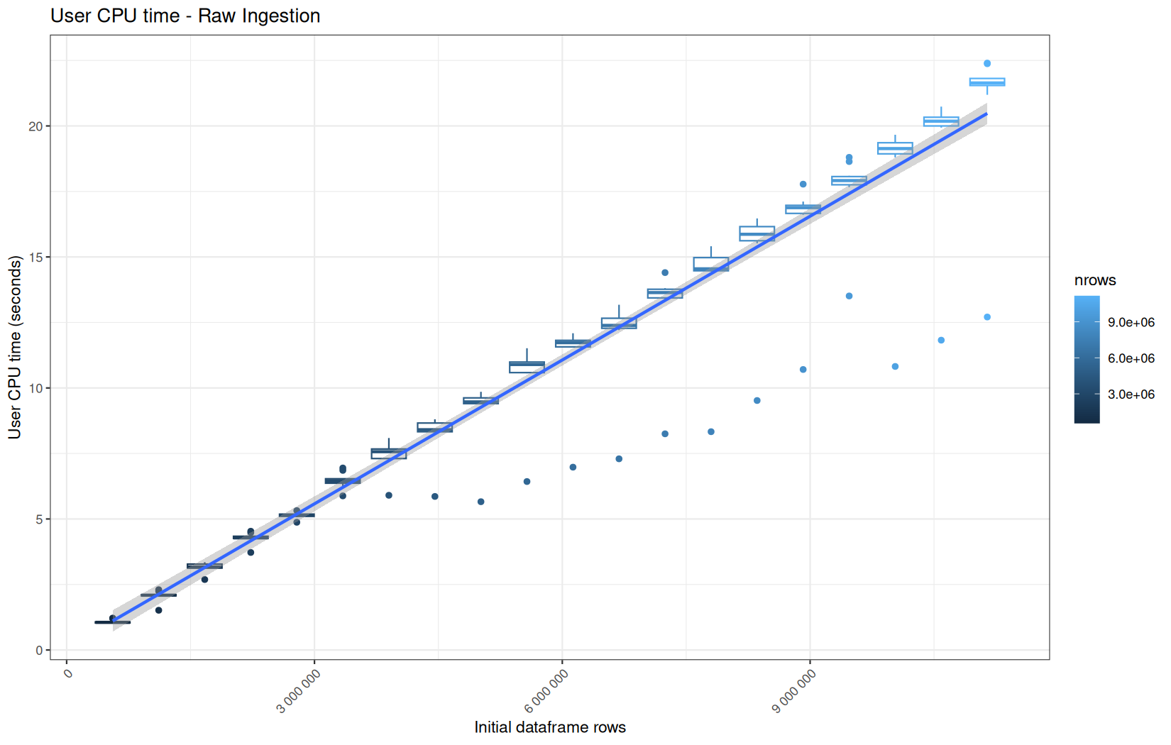

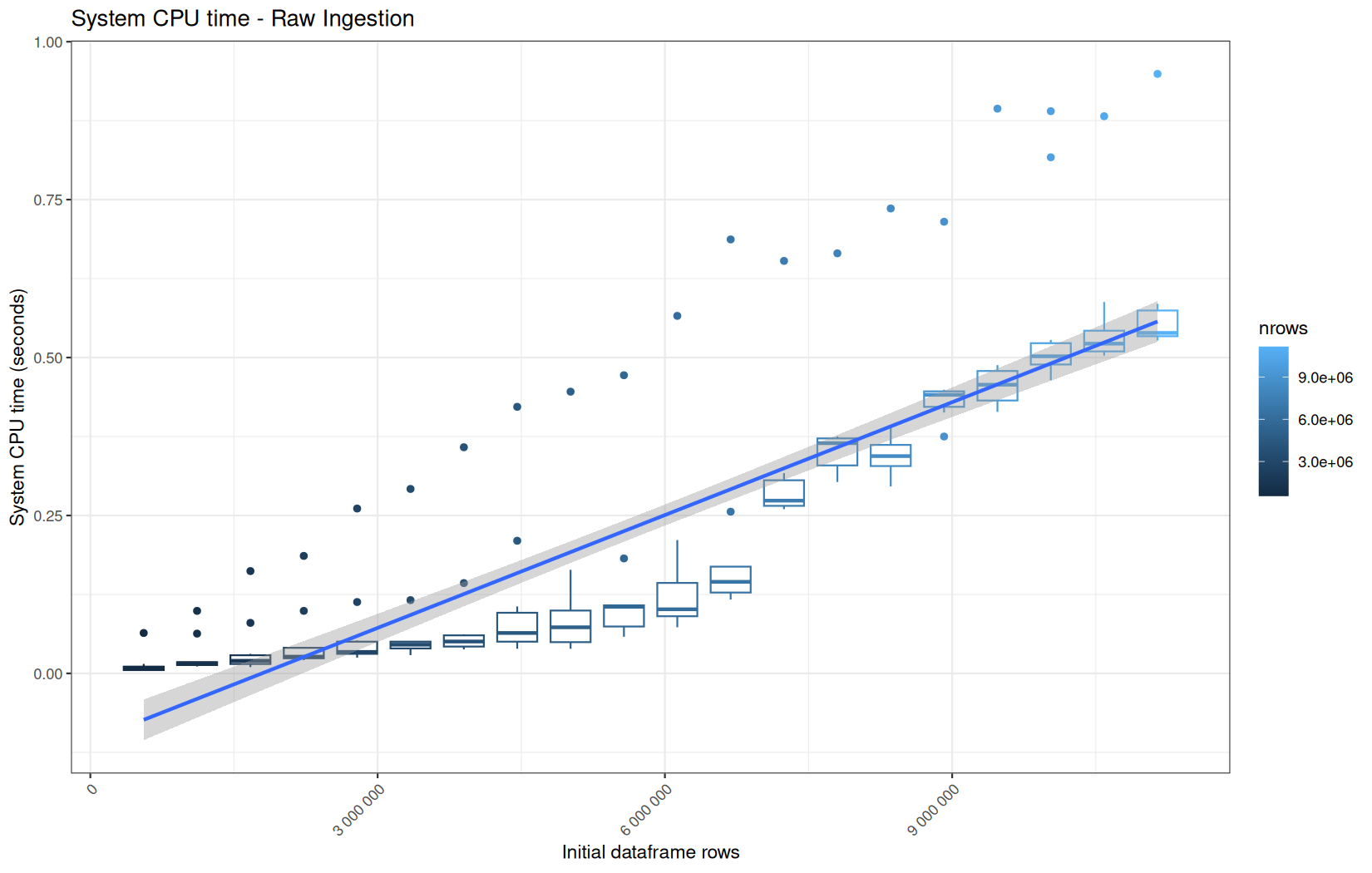
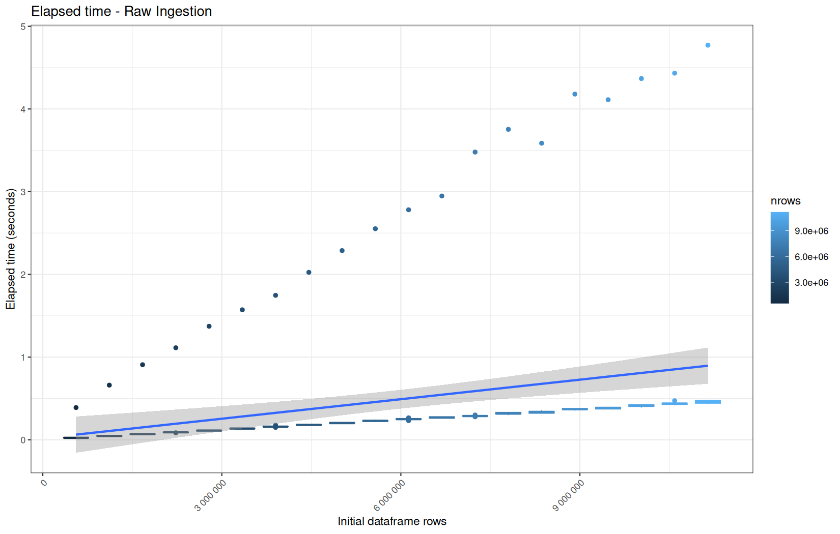
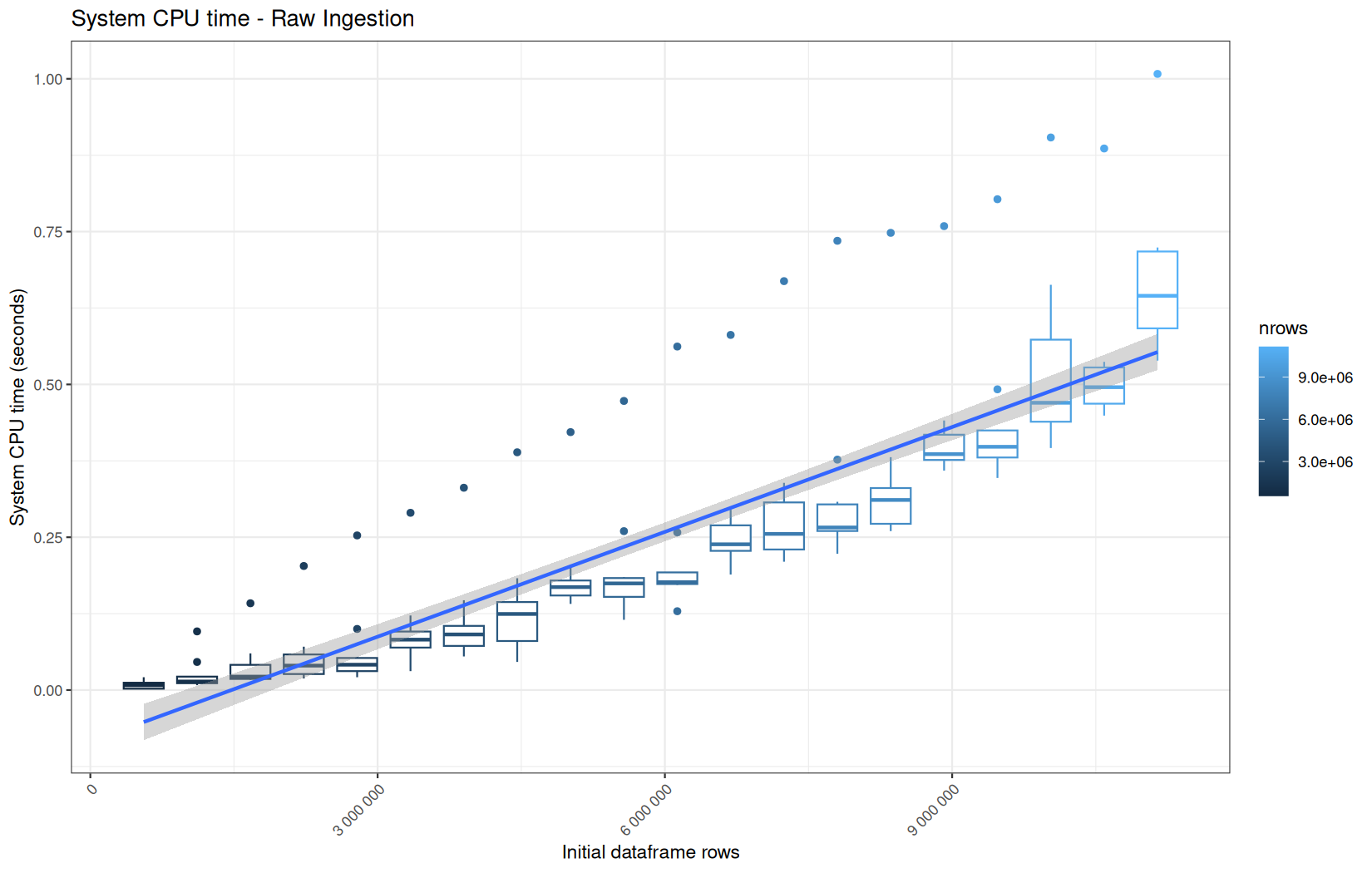
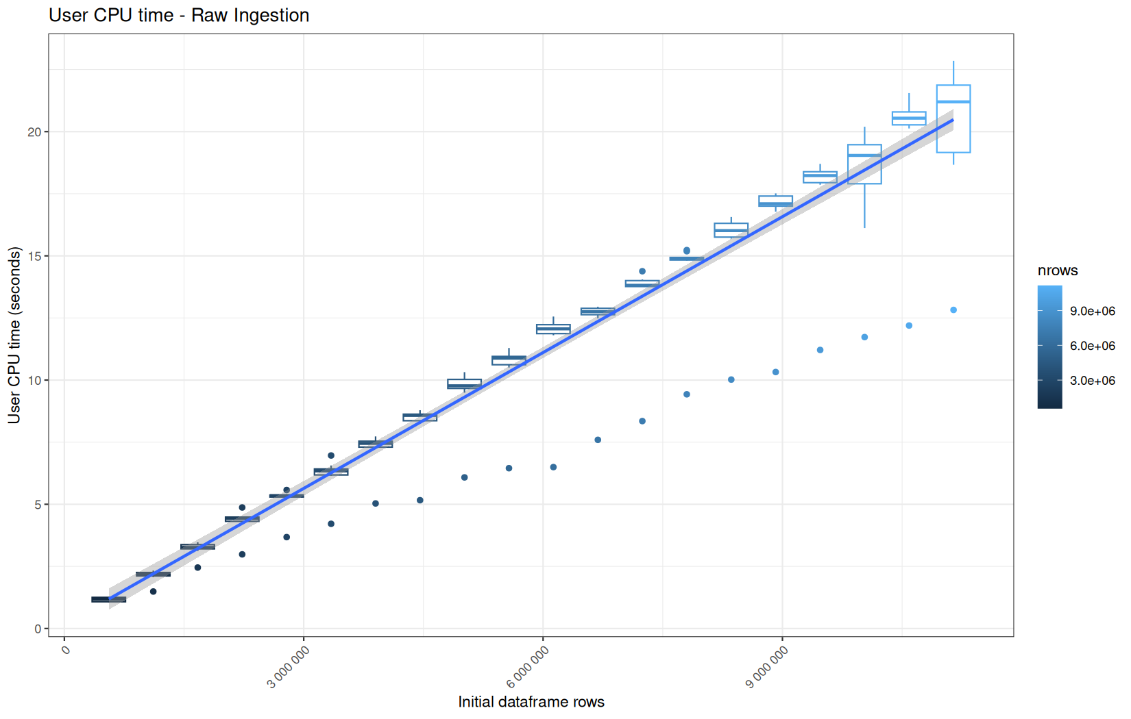
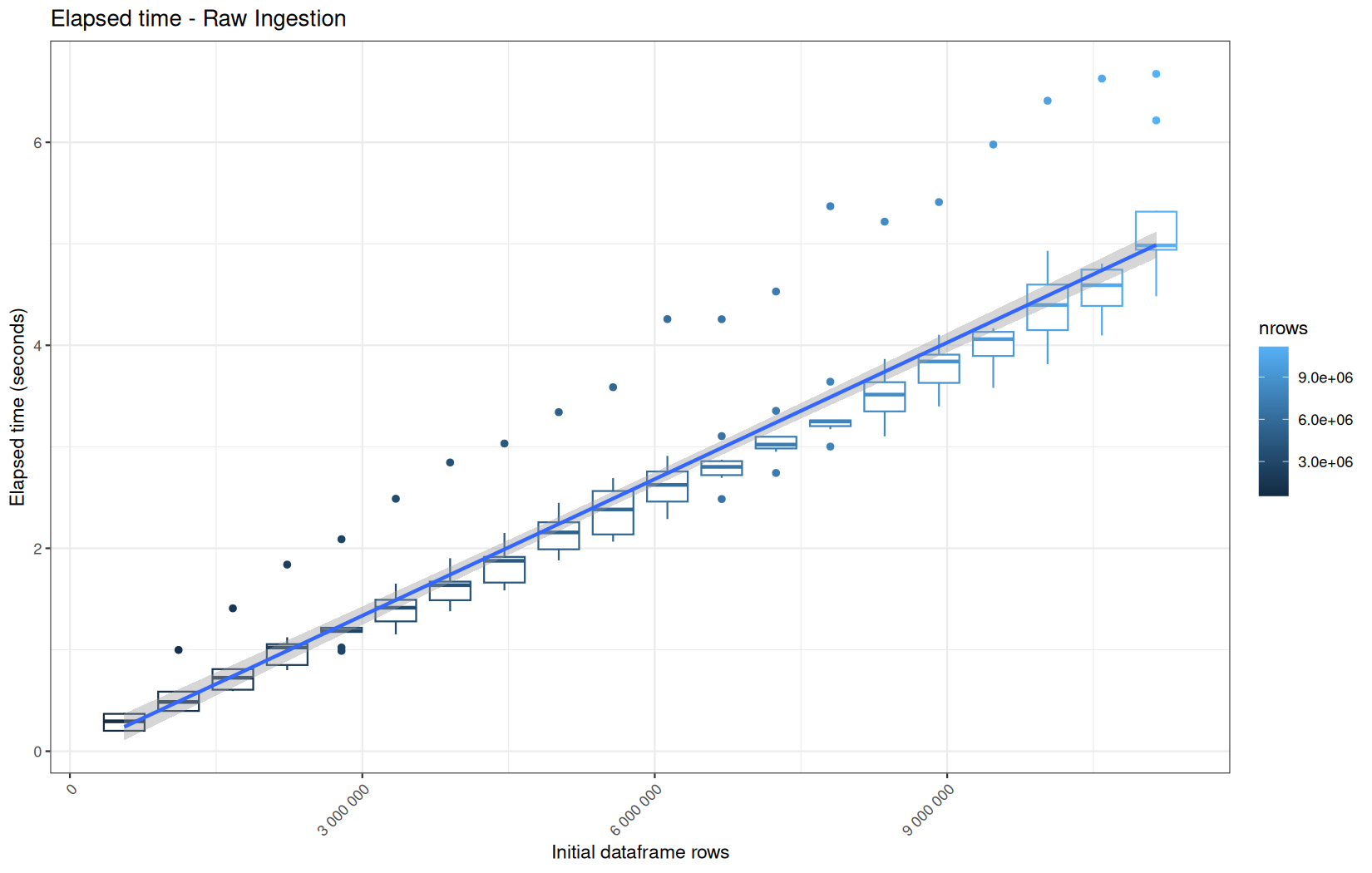
For fread one, we clearly see that the operation is multithreaded because the user time is lager than the elapsed time.
In a less intensive way we can also see it in readr and vroom.
We also note that readr and vroom are very similar.
In fact that's normal, because since readr version 2.0, it uses the same ingestion backend as vroom, but obviously not same policy in term of materialization ( expr is evaluated at different when needed in vroom ).
By the way since readr 2.1.0 we have the lazy option.
options(readr.read_lazy = TRUE)
readr::read_tsv(...)
So the thing we can ask is, at this point are the coumn yet materialized with as.data.table or still lazy promises ?
For that we will do:
log_step("RAW Ingestion", {
df <- data.table::as.data.table(vroom::vroom(
file_path,
delim = "\t",
col_names = c("ip", "ts", "target", "status", "ua"),
col_types = vroom::cols(
ip = vroom::col_character(),
ts = vroom::col_double(),
target = vroom::col_character(),
status = vroom::col_integer(),
ua = vroom::col_character()
),
progress = FALSE
))
})
cat("\n ip: ")
.Internal(inspect(df$ip))
cat("\n ts: ")
.Internal(inspect(df$ts))
cat("\n target: ")
.Internal(inspect(df$target))
cat("\n status: ")
.Internal(inspect(df$status))
cat("\n ua: ")
.Internal(inspect(df$ua))
cat("\n #### \n ")
And same for readr.
We see those reslts:
ip: @59068a95f8e0 16 STRSXP g1c7 [MARK,REF(4)] (len=557230, tl=0)
@59068901c5f8 09 CHARSXP g1c2 [MARK,REF(111),gp=0x60] [ASCII] [cached] "63.245.218.50"
@59068901c5f8 09 CHARSXP g1c2 [MARK,REF(111),gp=0x60] [ASCII] [cached] "63.245.218.50"
@59068901c5f8 09 CHARSXP g1c2 [MARK,REF(111),gp=0x60] [ASCII] [cached] "63.245.218.50"
@59068901c5f8 09 CHARSXP g1c2 [MARK,REF(111),gp=0x60] [ASCII] [cached] "63.245.218.50"
@59068901c5f8 09 CHARSXP g1c2 [MARK,REF(111),gp=0x60] [ASCII] [cached] "63.245.218.50"
...
ts: @59068985e1f0 14 REALSXP g1c7 [MARK,REF(4)] (len=557230, tl=0) 1.77996e+09,1.77996e+09,1.77996e+09,1.77996e+09,1.77996e+09,...
target: @59068b6209f0 16 STRSXP g1c7 [MARK,REF(4)] (len=557230, tl=0)
@59068716b848 09 CHARSXP g1c2 [MARK,REF(65535),gp=0x60] [ASCII] [cached] "/index.html"
@590687169928 09 CHARSXP g1c3 [MARK,REF(15871),gp=0x60,ATT] [ASCII] [cached] "/assets/css/font.css"
@590687169978 09 CHARSXP g1c3 [MARK,REF(15901),gp=0x60,ATT] [ASCII] [cached] "/assets/css/theme.css"
@5906871699c8 09 CHARSXP g1c3 [MARK,REF(15961),gp=0x60] [ASCII] [cached] "/assets/css/style.css"
@590687169a18 09 CHARSXP g1c3 [MARK,REF(13741),gp=0x60,ATT] [ASCII] [cached] "/assets/js/main.js"
...
status: @590689ebea90 13 INTSXP g0c7 [REF(4)] (len=557230, tl=0) 200,200,200,200,200,...
ua: @59068bea1550 16 STRSXP g0c7 [REF(4)] (len=557230, tl=0)
@590687183c38 09 CHARSXP g1c5 [MARK,REF(65535),gp=0x60,ATT] [ASCII] [cached] "Mozilla/5.0 (X11; Linux x86_64; rv:150.0) Gecko/20100101 Firefox/150.0"
@590687183c38 09 CHARSXP g1c5 [MARK,REF(65535),gp=0x60,ATT] [ASCII] [cached] "Mozilla/5.0 (X11; Linux x86_64; rv:150.0) Gecko/20100101 Firefox/150.0"
@590687183c38 09 CHARSXP g1c5 [MARK,REF(65535),gp=0x60,ATT] [ASCII] [cached] "Mozilla/5.0 (X11; Linux x86_64; rv:150.0) Gecko/20100101 Firefox/150.0"
@590687183c38 09 CHARSXP g1c5 [MARK,REF(65535),gp=0x60,ATT] [ASCII] [cached] "Mozilla/5.0 (X11; Linux x86_64; rv:150.0) Gecko/20100101 Firefox/150.0"
@590687183c38 09 CHARSXP g1c5 [MARK,REF(65535),gp=0x60,ATT] [ASCII] [cached] "Mozilla/5.0 (X11; Linux x86_64; rv:150.0) Gecko/20100101 Firefox/150.0"
...
For both readr and vroom variant.
So none of them is ALTREP, meaning al of them is fuly materialized.
| Column | Declared type | readr internal type |
vroom internal type |
Interpretation |
|---|---|---|---|---|
ip |
character | STRSXP |
STRSXP |
Materialized R character vector containing references to cached CHARSXP strings |
ts |
double | REALSXP |
REALSXP |
Materialized contiguous double vector |
target |
character | STRSXP |
STRSXP |
Materialized R character vector containing references to cached CHARSXP strings |
status |
integer | INTSXP |
INTSXP |
Materialized contiguous integer vector |
ua |
character | STRSXP |
STRSXP |
Materialized R character vector containing references to cached CHARSXP strings |
That is surely due to as.data.table.
We will confirm thatlater with dplyr variant.
dplyr
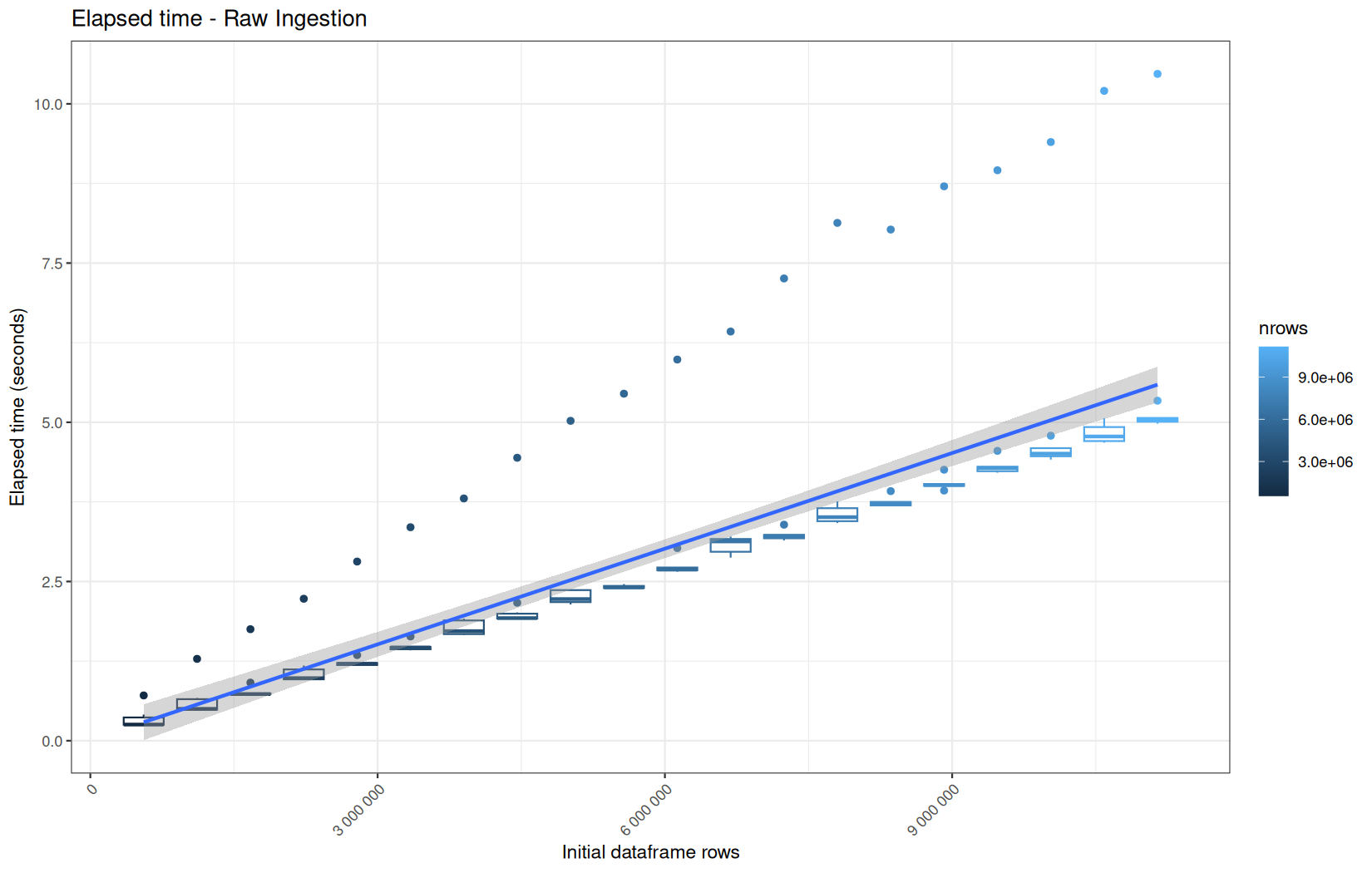
We see that here vroom clearly wins, surely because it is really being lazy here.
Also, here we totally see that all operations are multithreaded.
For the vroom path, we see that the cold-sart are above the median in elapsed_time, but we do not see it in user_time neither at this scale on system_time. This mean the operation is just waiting for someting not doing any CPU work.
It's normal because that is the cold-start:
-
file not warm in OS page cache
-
vroom builds lazy/indexed representation
-
OS has to fetch file pages
In fact, we have this effect on all paths, it is just more visible here because the difference is larger due to the execution time of the native vroom path being very fast.
On the fread path, the conversion cost to data.table was added on top of ingestion, and this added cost may scale differently from the ingestion cost, so it could have hide/dilute the visible multithreading factor.
Now for the output of this code:
cat("\n ip: ")
.Internal(inspect(df$ip))
cat("\n ts: ")
.Internal(inspect(df$ts))
cat("\n target: ")
.Internal(inspect(df$target))
cat("\n status: ")
.Internal(inspect(df$status))
cat("\n ua: ")
.Internal(inspect(df$ua))
cat("\n #### \n ")
For readr we have pretty much the same thing as before:
ip: @5fe71b8a8460 16 STRSXP g0c7 [REF(8)] (len=557230, tl=0)
@5fe71a9f1b08 09 CHARSXP g1c2 [MARK,REF(148),gp=0x60] [ASCII] [cached] "63.245.218.50"
@5fe71a9f1b08 09 CHARSXP g1c2 [MARK,REF(148),gp=0x60] [ASCII] [cached] "63.245.218.50"
@5fe71a9f1b08 09 CHARSXP g1c2 [MARK,REF(148),gp=0x60] [ASCII] [cached] "63.245.218.50"
@5fe71a9f1b08 09 CHARSXP g1c2 [MARK,REF(148),gp=0x60] [ASCII] [cached] "63.245.218.50"
@5fe71a9f1b08 09 CHARSXP g1c2 [MARK,REF(148),gp=0x60] [ASCII] [cached] "63.245.218.50"
...
ts: @5fe71bce8a10 14 REALSXP g0c7 [REF(8)] (len=557230, tl=0) 1.77996e+09,1.77996e+09,1.77996e+09,1.77996e+09,1.77996e+09,...
target: @5fe71c128fc0 16 STRSXP g0c7 [REF(8)] (len=557230, tl=0)
@5fe71ae15f68 09 CHARSXP g1c2 [MARK,REF(65535),gp=0x60] [ASCII] [cached] "/index.html"
@5fe71a9f9258 09 CHARSXP g1c3 [MARK,REF(21161),gp=0x60,ATT] [ASCII] [cached] "/assets/css/font.css"
@5fe71a9f9208 09 CHARSXP g1c3 [MARK,REF(21201),gp=0x60,ATT] [ASCII] [cached] "/assets/css/theme.css"
@5fe71a9f91b8 09 CHARSXP g1c3 [MARK,REF(21281),gp=0x60] [ASCII] [cached] "/assets/css/style.css"
@5fe71a9f9168 09 CHARSXP g1c3 [MARK,REF(18321),gp=0x60,ATT] [ASCII] [cached] "/assets/js/main.js"
...
status: @5fe71c569570 13 INTSXP g0c7 [REF(8)] (len=557230, tl=0) 200,200,200,200,200,...
ua: @5fe71c789860 16 STRSXP g0c7 [REF(8)] (len=557230, tl=0)
@5fe71ae21348 09 CHARSXP g1c5 [MARK,REF(65535),gp=0x60,ATT] [ASCII] [cached] "Mozilla/5.0 (X11; Linux x86_64; rv:150.0) Gecko/20100101 Firefox/150.0"
@5fe71ae21348 09 CHARSXP g1c5 [MARK,REF(65535),gp=0x60,ATT] [ASCII] [cached] "Mozilla/5.0 (X11; Linux x86_64; rv:150.0) Gecko/20100101 Firefox/150.0"
@5fe71ae21348 09 CHARSXP g1c5 [MARK,REF(65535),gp=0x60,ATT] [ASCII] [cached] "Mozilla/5.0 (X11; Linux x86_64; rv:150.0) Gecko/20100101 Firefox/150.0"
@5fe71ae21348 09 CHARSXP g1c5 [MARK,REF(65535),gp=0x60,ATT] [ASCII] [cached] "Mozilla/5.0 (X11; Linux x86_64; rv:150.0) Gecko/20100101 Firefox/150.0"
@5fe71ae21348 09 CHARSXP g1c5 [MARK,REF(65535),gp=0x60,ATT] [ASCII] [cached] "Mozilla/5.0 (X11; Linux x86_64; rv:150.0) Gecko/20100101 Firefox/150.0"
...
But for vroom:
ip: @650382851880 16 STRSXP g0c0 [REF(65535)] vroom_chr (len=557230, materialized=F)
ts: @650382851bc8 14 REALSXP g0c0 [REF(65535)] vroom_dbl (len=557230, materialized=F)
target: @650382851fb8 16 STRSXP g0c0 [REF(65535)] vroom_chr (len=557230, materialized=F)
status: @65038284e620 13 INTSXP g0c0 [REF(65535)] vroom_int (len=557230, materialized=F)
ua: @65038284e9d8 16 STRSXP g0c0 [REF(65535)] vroom_chr (len=557230, materialized=F)
That is very interesting:
| Function | Internal column representation after ingestion | Materialization state | Interpretation |
|---|---|---|---|
vroom::vroom() |
vroom_chr, vroom_dbl, vroom_int |
materialized=F |
Lazy ALTREP columns. The file has been indexed, but column values have not yet been fully parsed into ordinary R vectors. |
readr::read_tsv() |
STRSXP, REALSXP, INTSXP |
Fully materialized | Ordinary R vectors. Character, double, and integer values have already been parsed and stored in memory. |
And also confirming that as.data.table was forcing the column materialization.
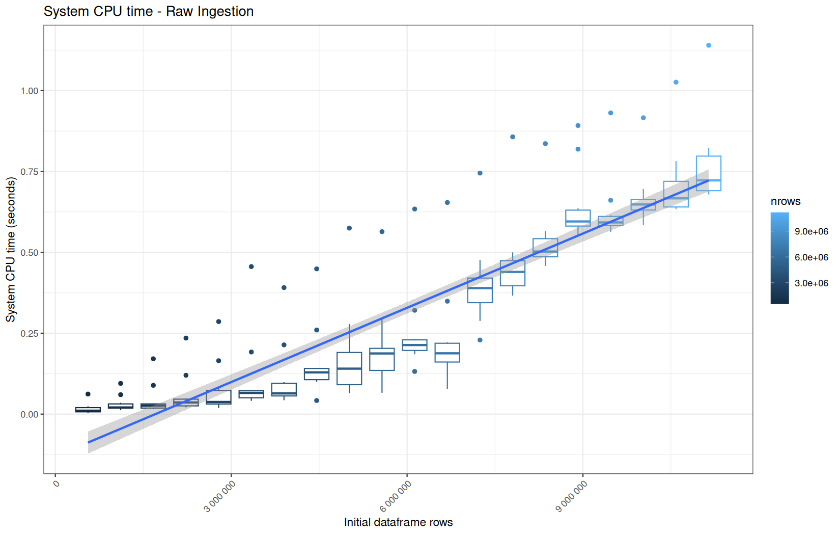
Conclusion
Across all plots, raw ingestion time remains relatively stable across iterations.
However, in each group of ten consecutive runs, we observe exactly one large outlier.
This outlier corresponds to the first, cold execution, during which the file is not yet present in the operating system’s page cache.
One-time initialization costs is incurred.
The following nine runs benefit from a warm cache and already initialized runtime structures, resulting in much lower and more stable execution times.
Memory consumption
data.table
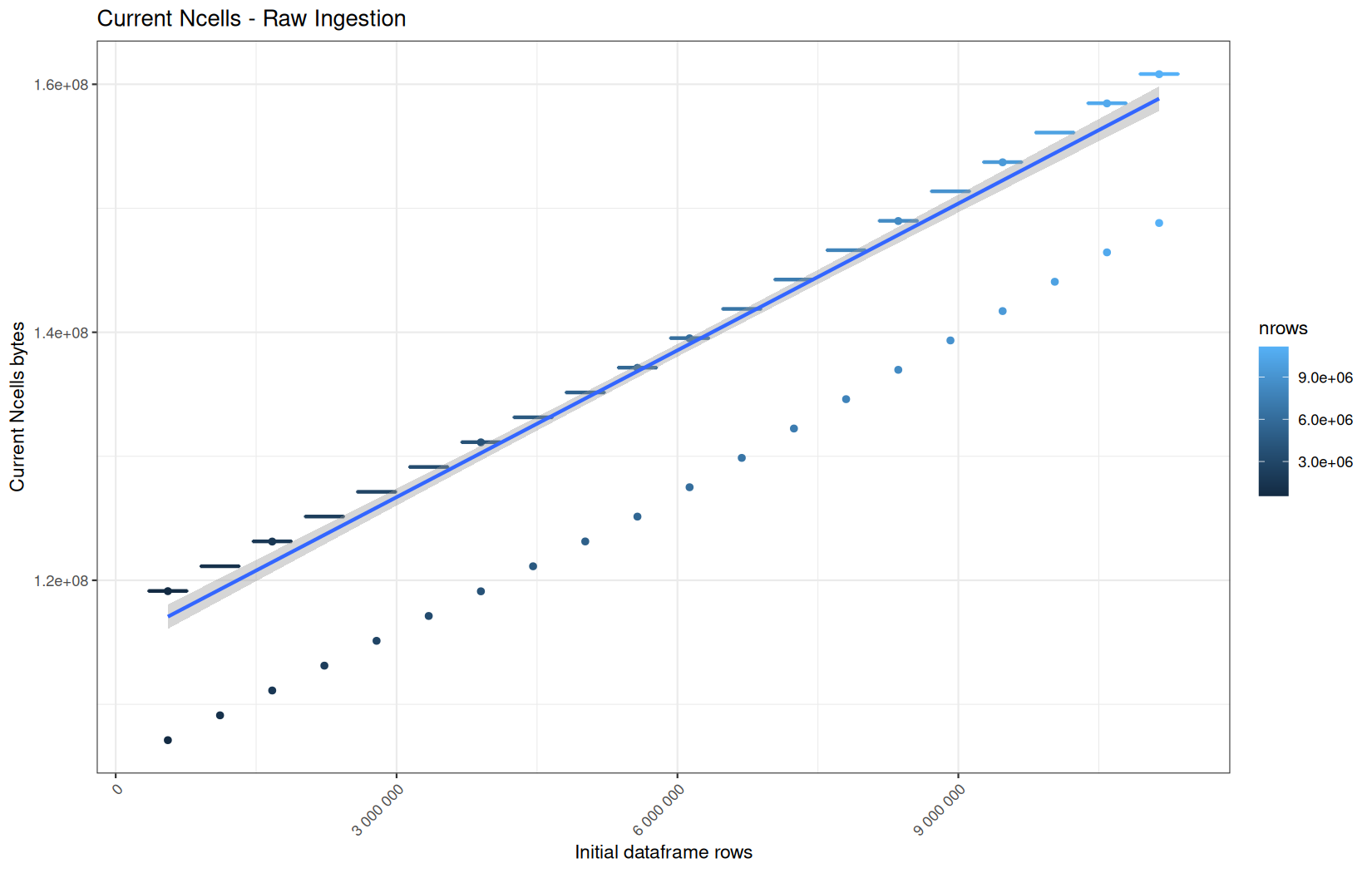
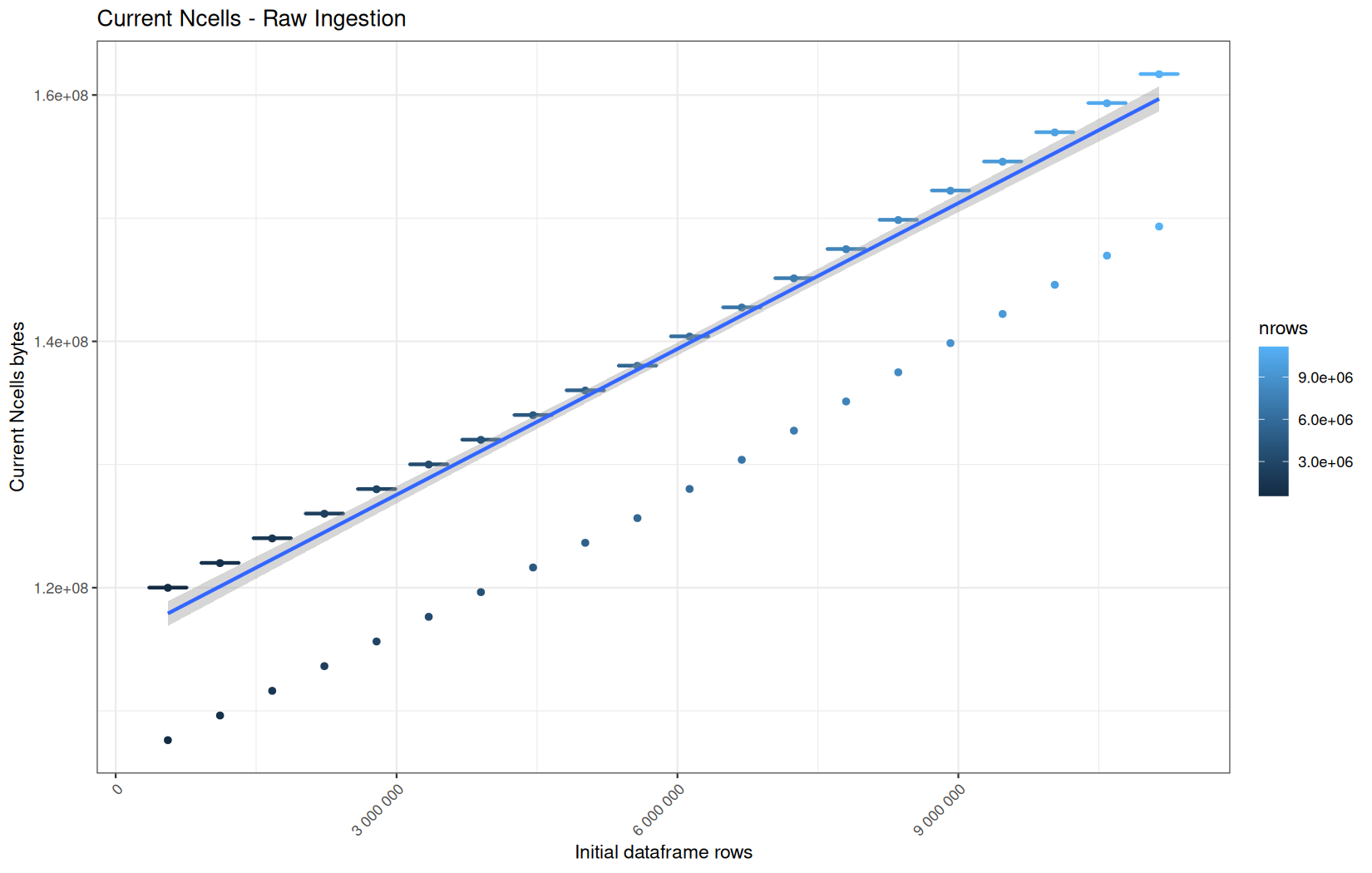
Current NCells:
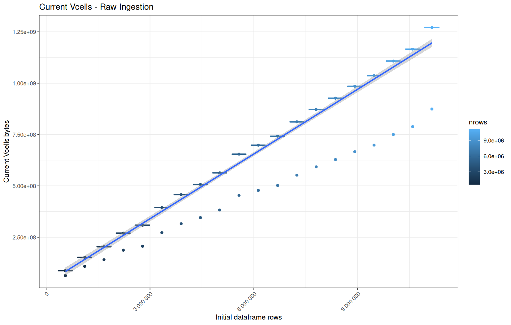
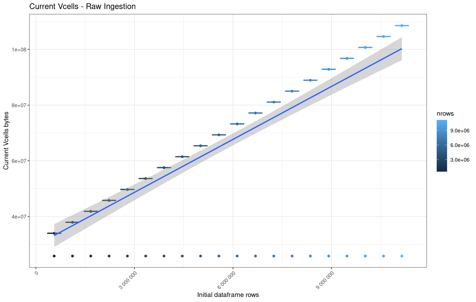
Current VCells:

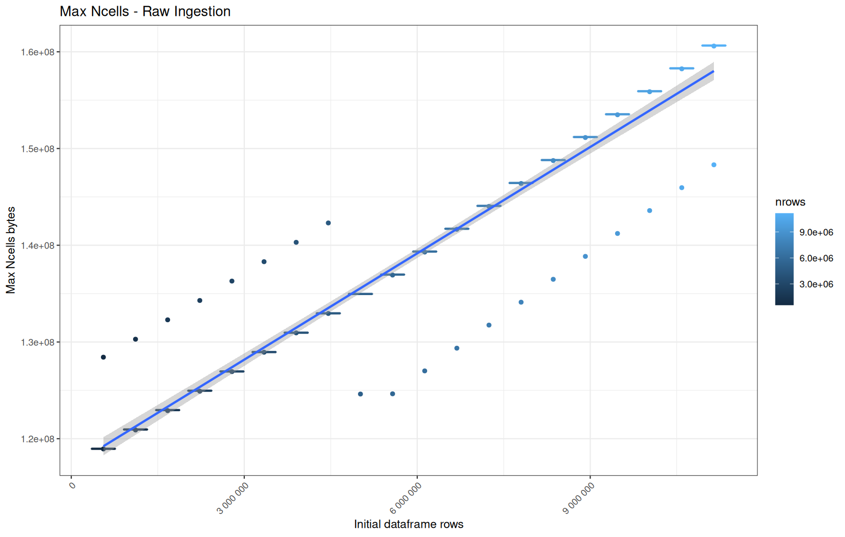
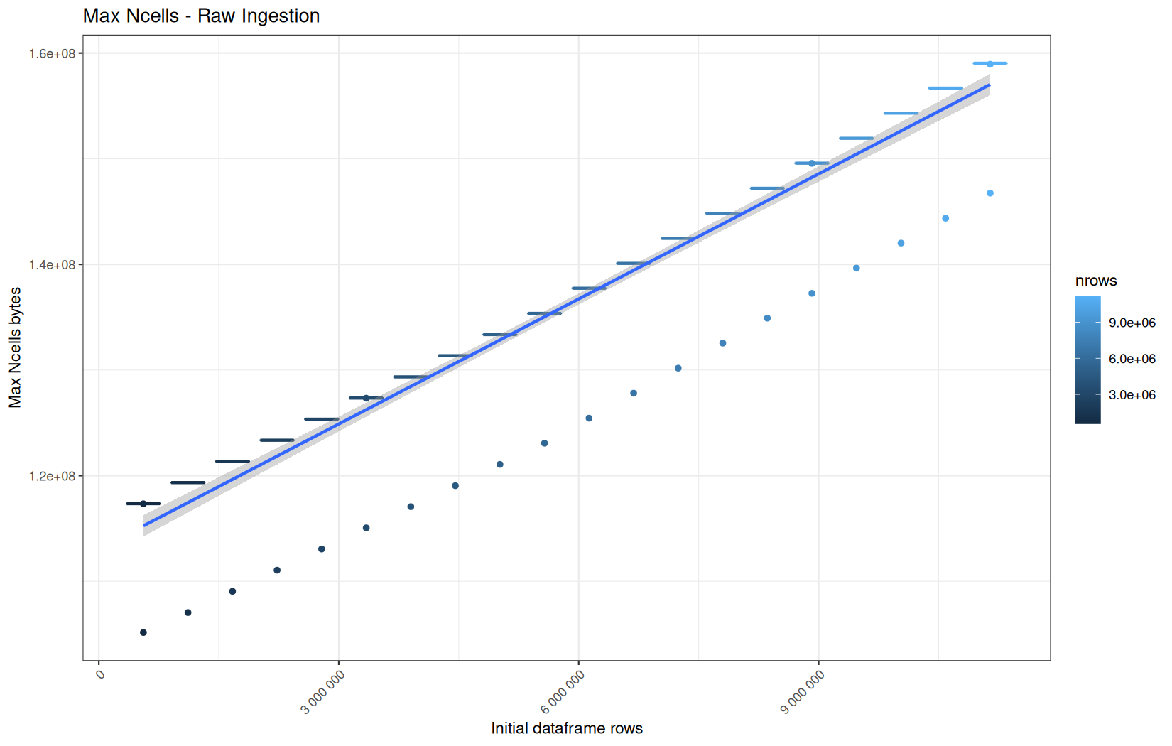
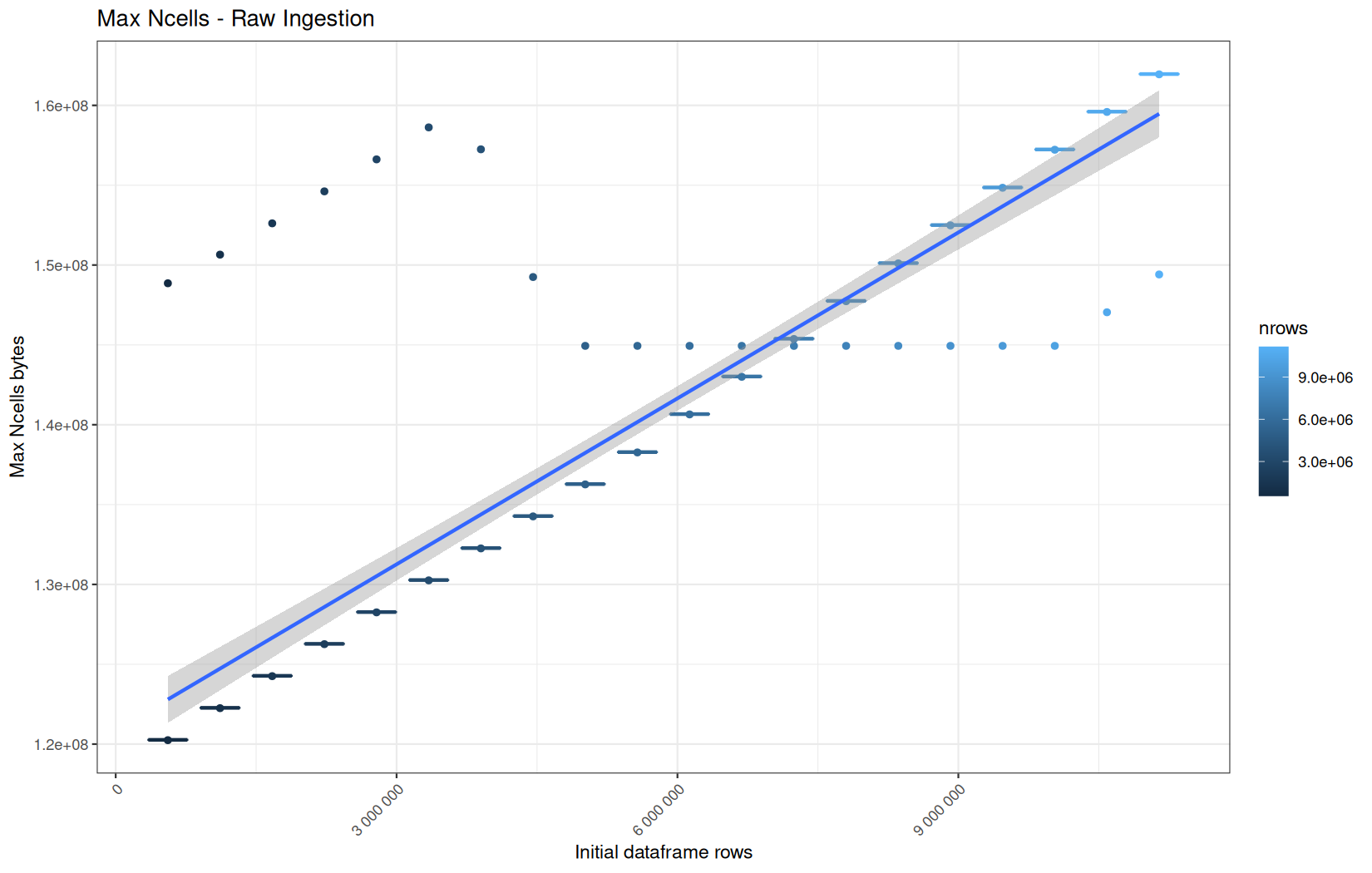
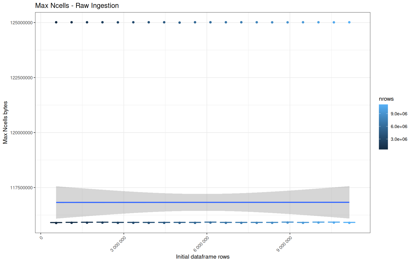
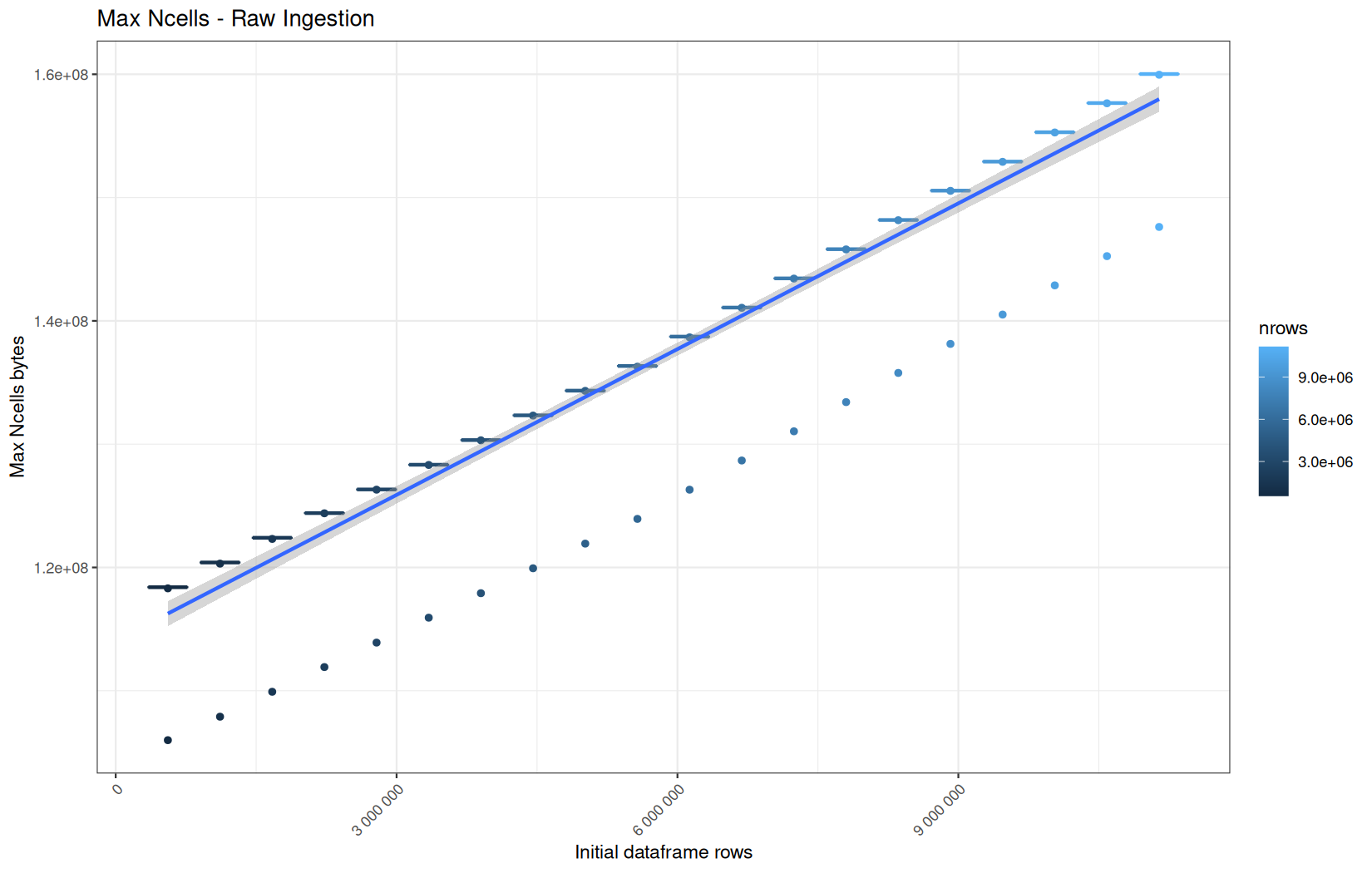
Max NCells:

Max VCells:

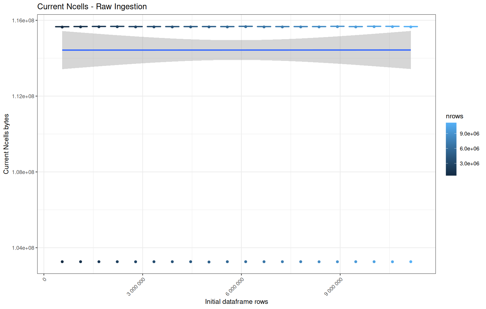
Current NCells:

Current VCells:

Max NCells:
Max VCells:

Current NCells:

Current VCells:
Max NCells:
Max VCells:

In short, memory usage increases approximately linearly with the number of rows.
For the same benchmark run, VCells usage is roughly an order of magnitude higher than NCells usage. This is expected because the pipeline mainly stores and manipulates column data in ordinary R vectors, so most of the memory is consumed by vector payloads rather than by node-based language objects or internal metadata.
For most implementations, current and maximum memory usage remain pretty close. This indicates that peak memory consumption does not rise far above the amount of memory still in use at the end of the measured operation.
However, for vroom and readr, the gap between current_vcells and max_vcells is larger. Their max_vcells values have a significant higher value.
This suggests that these ingestion paths allocate more temporary vector memory during execution, some of which is released before the final current_vcells measurement is taken.
Also, we generally see that the cold start iteration for each benchmark are below the median memory consumption and increases at a lower rate.
The cold run may take longer while still reaching a lower absolute memory peak because it is the first execution in a relatively clean R process. The following browser reloads reuse the same R process, in which some runtime structures, cached strings / vectors..., package state, and other allocations may remain present.
Consequently, later runs begin from a higher memory baseline.
Since gc(reset = TRUE) resets the max used counter to the current memory usage rather than resetting memory usage to zero, subsequent runs can report higher absolute current/max_ncells and current/max_vcells values even when their execution times are lower.
The cold run is therefore slower because of initialization and filesystem-cache effects, but lower in absolute memory usage because less state has accumulated in the R process at that point.
dplyr
Current NCells:
Current VCells:

Max NCells:
Max VCells:

Current NCells:
Current VCells:
Max NCells:
Max VCells:

Current NCells:

Current VCells:

Max NCells:
Max VCells:

Regarding the lower-value outliers, this is the same explanation as before.
But first, we note that vroom is allocating susbstantially less (VCells), which is normal because it can be lazy here.
Also, the first native vroom ingestion run is measured before the process has ever materialized the dataset. It therefore reflects a very low lazy-object allocation floor.
After the dataframe has been materialized later in the pipeline, the R process is no longer in the same state. Even if gc(reset = TRUE) is called before the next run, only garbage collection and max-used counter reset happen, the R process itself is not restarted. Some initialized or still-reachable memory remains part of the baseline.
Therefore, the native vroom ingestion runs start from a higher warmed/materialized baseline, which explains why the first run is a low and constant outlier while the next runs are increasingly and higher.
We can conclude that vroom roughly does very low and constant allocations regardless of the file size. (because here the outliers tells the real story)
For its NCells we can also conclude the same thing.
But we can add that because cold start in max_ncells are higher but lower in current_ncells, the initialization of the ingestion backend requires some temporary more use of NCells. And we keep the same old fresh VS used R process explanation than before regarding why the cold start current_ncells values are lower (cached structures...).
Now, for fread.
We see that fread + tibble in current_vcells uses less memory (when we do not look at the cold start) than its native fread + data.table.
It is maybe not because fread allocates agressively for speed and data.table does not apply some sort of .shrink_to_fit(), but tibble does it.
Looking at the same metric for readr, we note the same pattern.
But still, it does not suggest that the tibble representation is more compact.
Even if in fact a tibble stores the raw column data in a fundamentally different way.
Both tibble and data.table ultimately store columns as R vectors.
And that the difference is more likely at the table-object level:
-
A
data.tablekeeps additional infrastructure to support by-reference mutation, fast column management, keys/indices, and internal self-reference behavior. -
A
tibbleis a simpler final container, so after reading the same data it can appear more compact in gc() measurements.
Because we can verify that running the following script:
library(lobstr)
library(data.table)
library(tibble)
tb <- readr::read_tsv("logs/out10.log", show_col_types = FALSE)
DT <- as.data.table(tb)
obj_size(tb)
obj_size(DT)
Result:
248.14 MB
248.13 MB
The lower Vcells in the tibble variant does not seem to come from the tibble object being more compact than the data.table object.
Direct object-size inspection shows both final objects are almost identical in memory size. Therefore, the observed Vcells difference is again more likely due to the noise of the R session.
So we must look at the cold-start.
They are the same for readr, but still less VCells usage in fread + tibble.
fread appears to use a speed-oriented allocation strategy, and the native data.table path may retain more allocation overhead in the R heap. When the result is converted to tibble, the final object graph can be simpler or cleaner, so fewer Vcells remain visible after gc(). Conceptually this looks like a compaction effect.
When it comes to readr, we see in both native path execution and with the data.table conversion that there is a very very weird correlation between the cold-start max_ncells values and the log-file size.
That is like a wave with a constant baseline.
So the largest amount of internal of temporary objects in readr increases with file size but is maybe bounded by the fact that it does not necessarily keep more of it alive simultaneously.
Conclusion
The memory usage is so similiar for the hot runs that the box-plots are literally conincident points.
But they tell another story than the cold-start, because there is still reachable cells by R by the time theay are reran.
The initialization of ingestion backends like vroom may create temporary memory peaks for NCells.
data.table forces materialization.
Note that the max_vcells and max_ncells could have varied if we did not used the lazy argument way which is just passing the expression directly into the conversion function, like:
df <- data.table::as.data.table(vroom::vroom(
file_path,
delim = "\t",
col_names = c("ip", "ts", "target", "status", "ua"),
col_types = vroom::cols(
ip = vroom::col_character(),
ts = vroom::col_double(),
target = vroom::col_character(),
status = vroom::col_integer(),
ua = vroom::col_character()
),
progress = FALSE
))
Where the expression wil be evaluated according to data.table::as.data.table, when it will need to get the actual value returned by the expression (eventually not too long after the call) .
Contrary to direclty evaluating the expression assigning it to a temporary value (it can be more predictible):
df <- vroom::vroom(
file_path,
delim = "\t",
col_names = c("ip", "ts", "target", "status", "ua"),
col_types = vroom::cols(
ip = vroom::col_character(),
ts = vroom::col_double(),
target = vroom::col_character(),
status = vroom::col_integer(),
ua = vroom::col_character()
),
progress = FALSE
)
df <- data.table::as.data.table(df)
First data-manipulations
Execution time
data.table
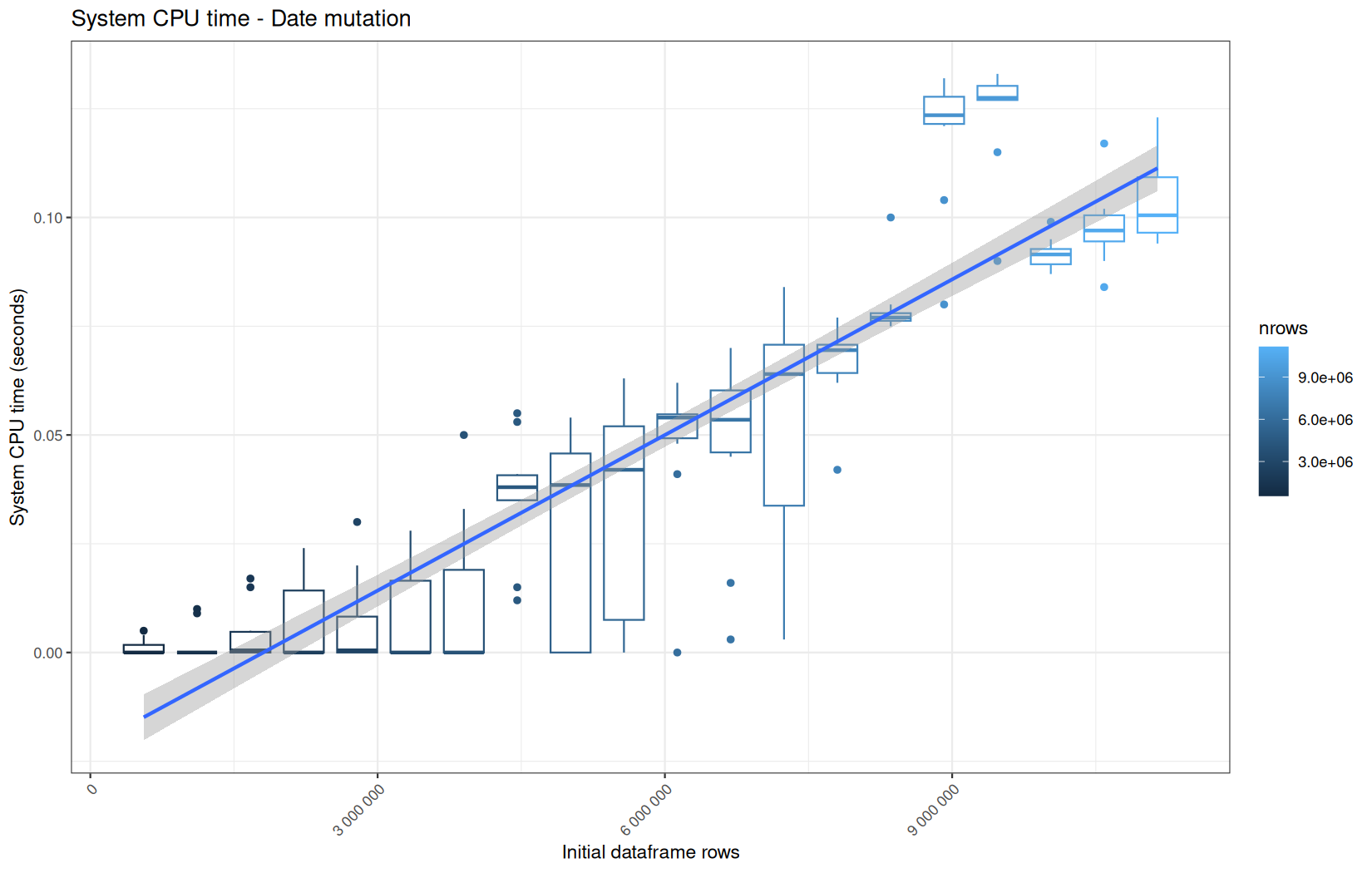
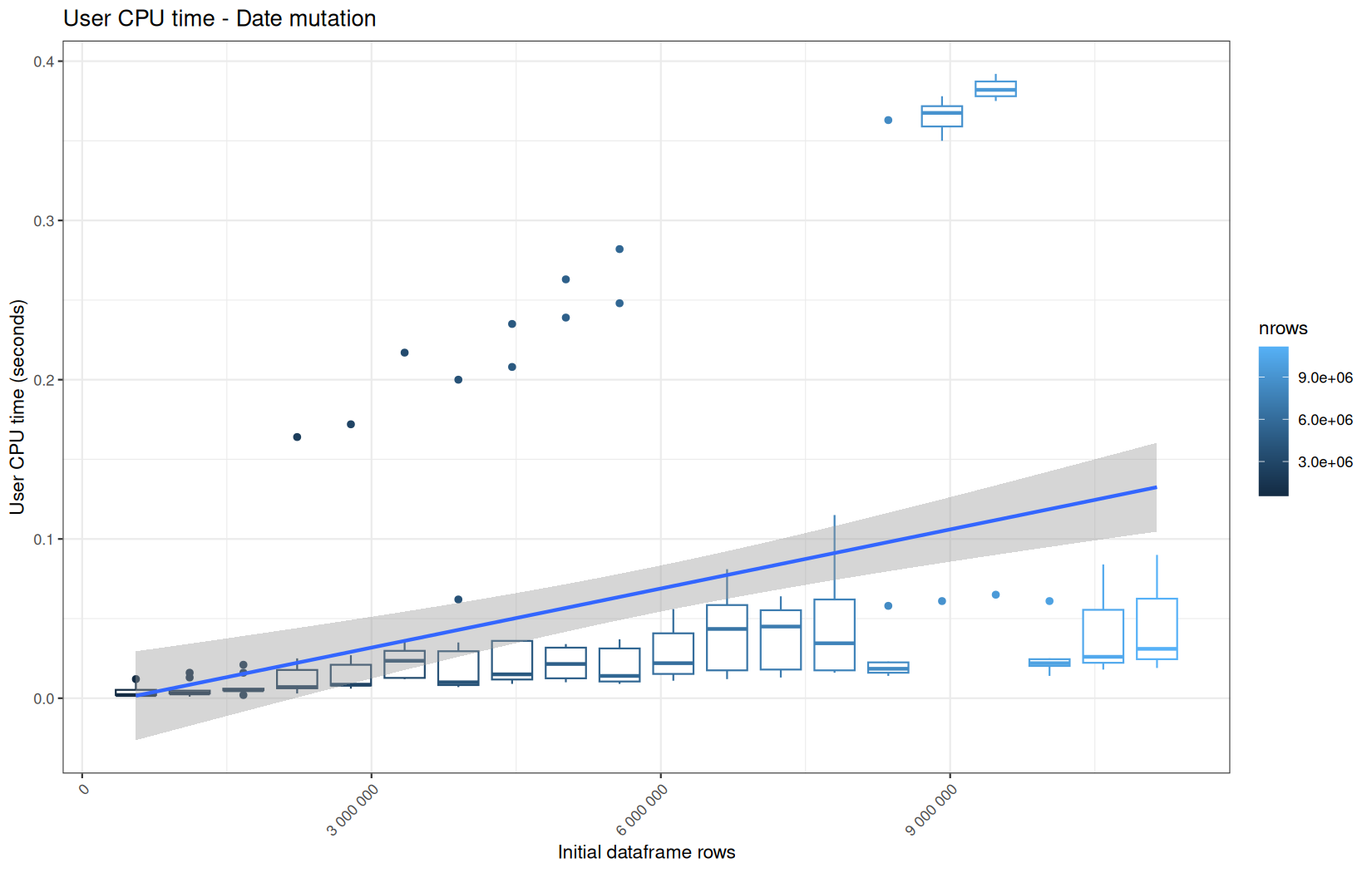
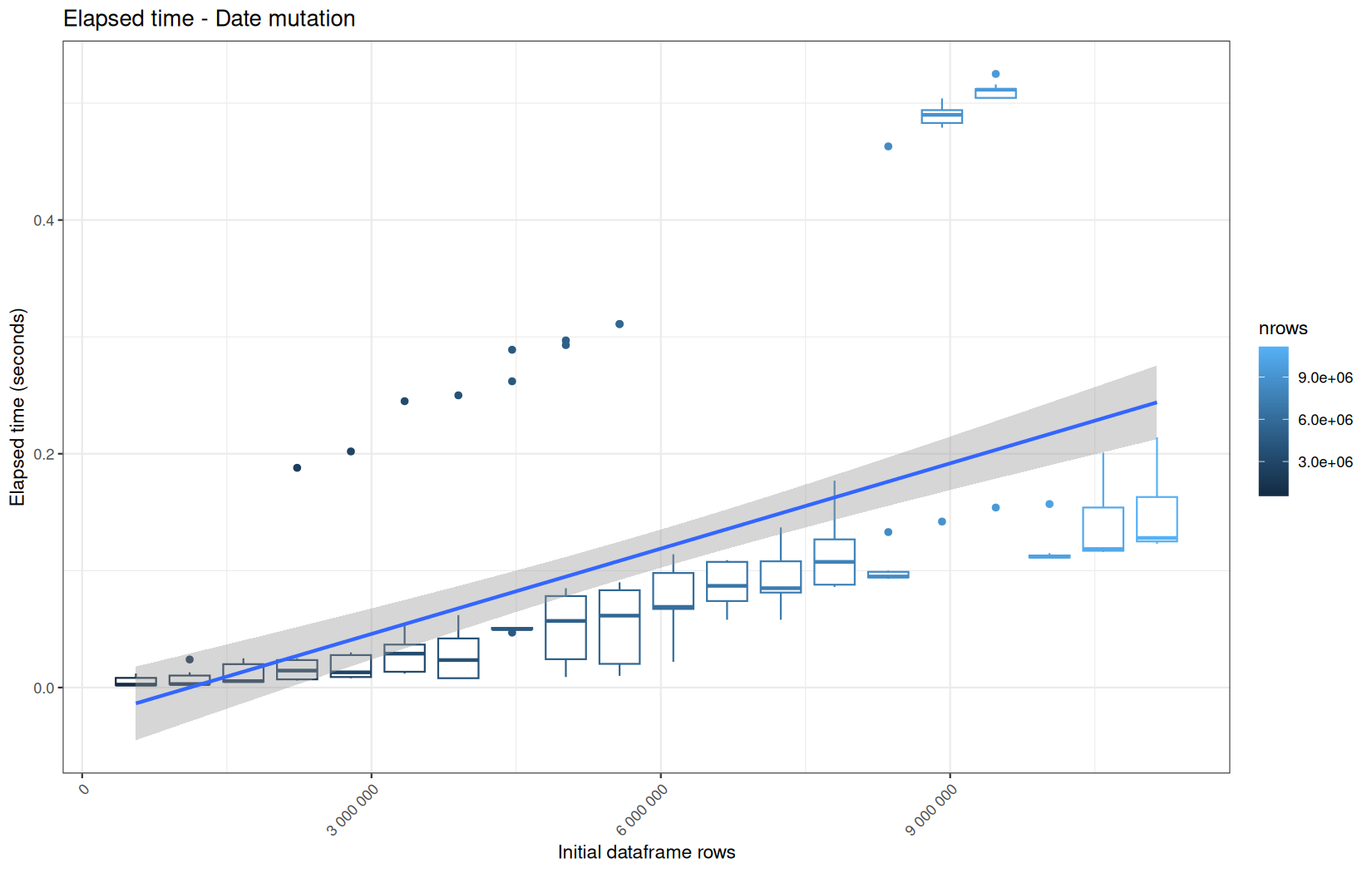
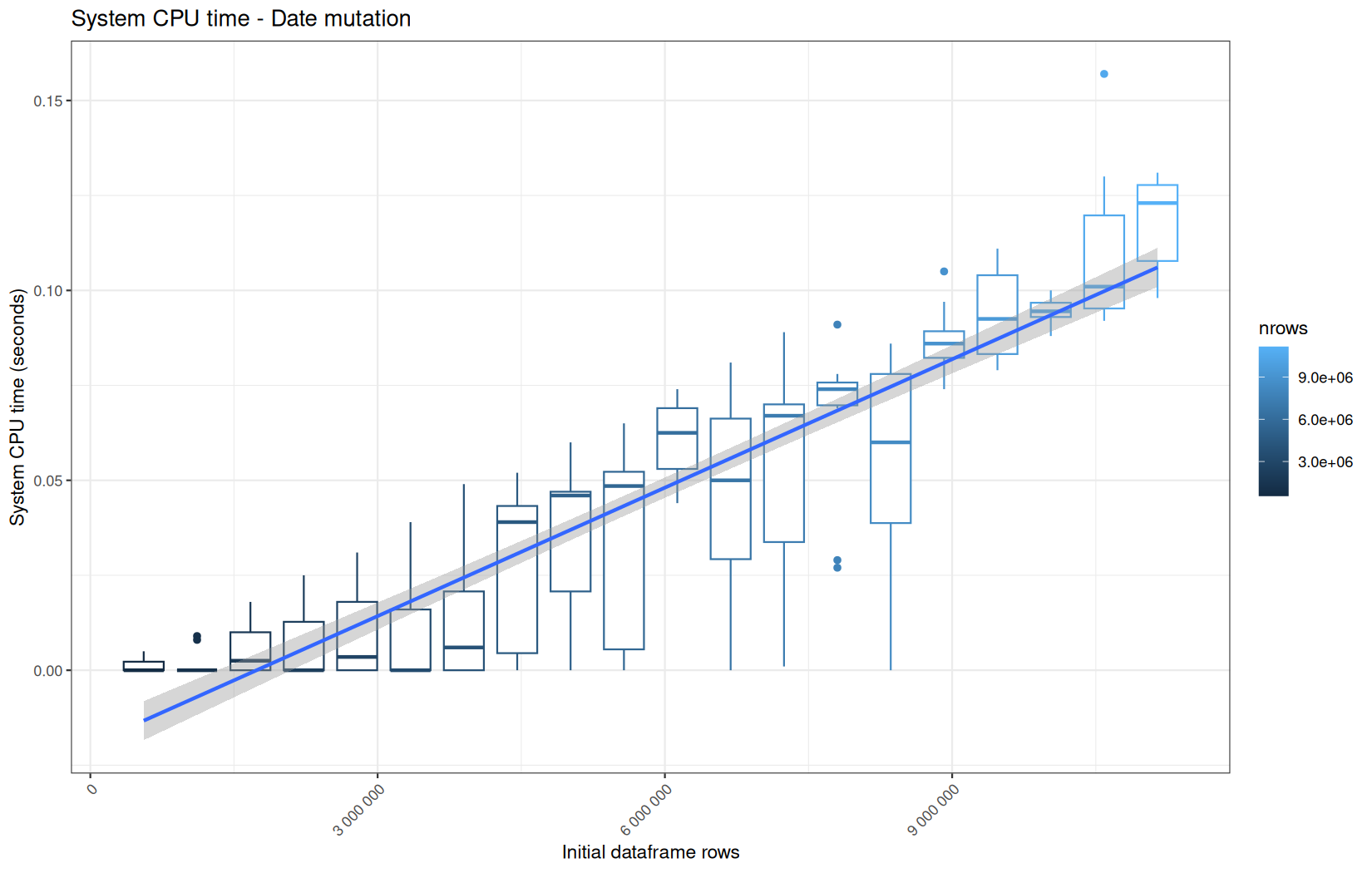
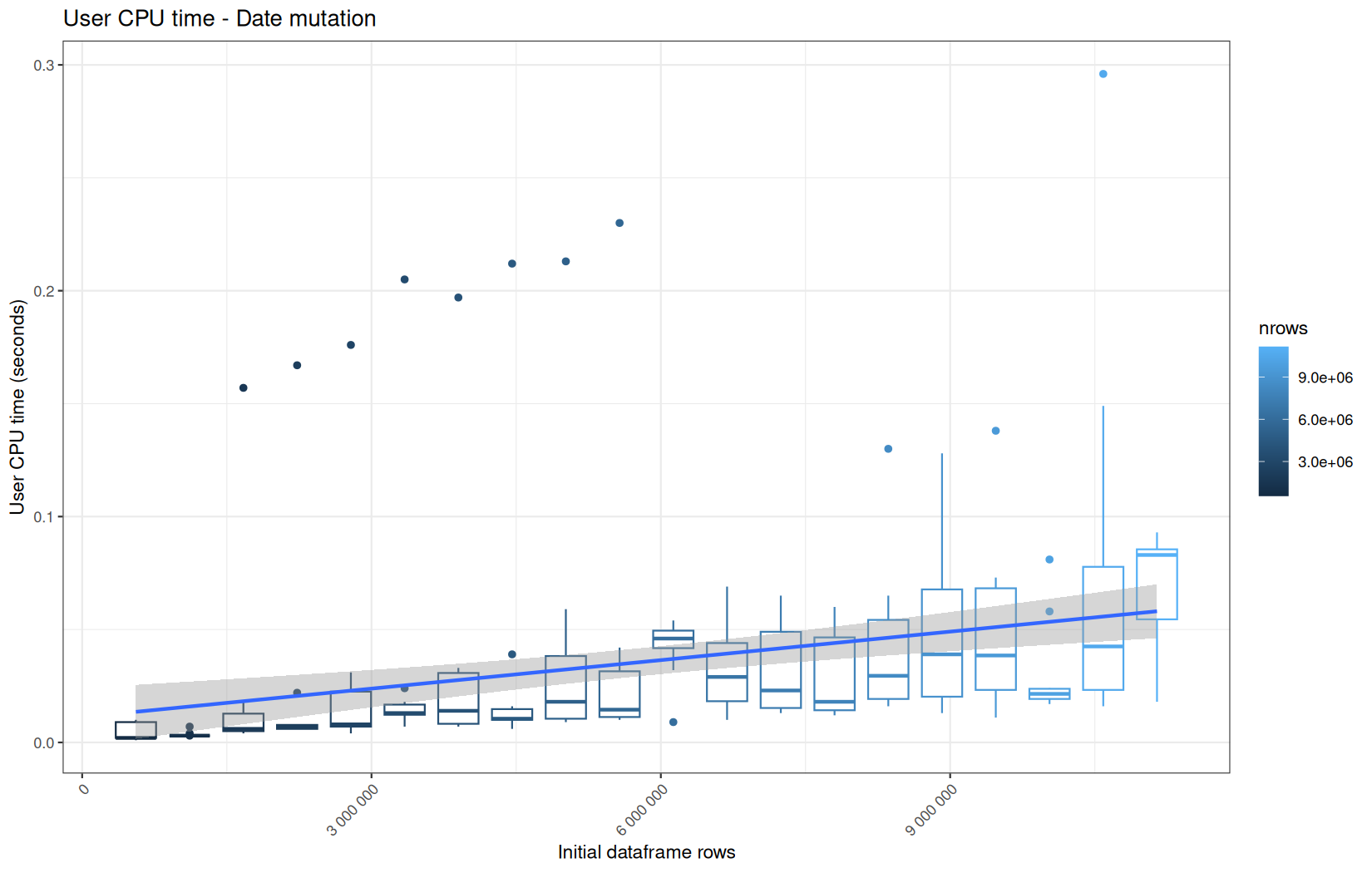
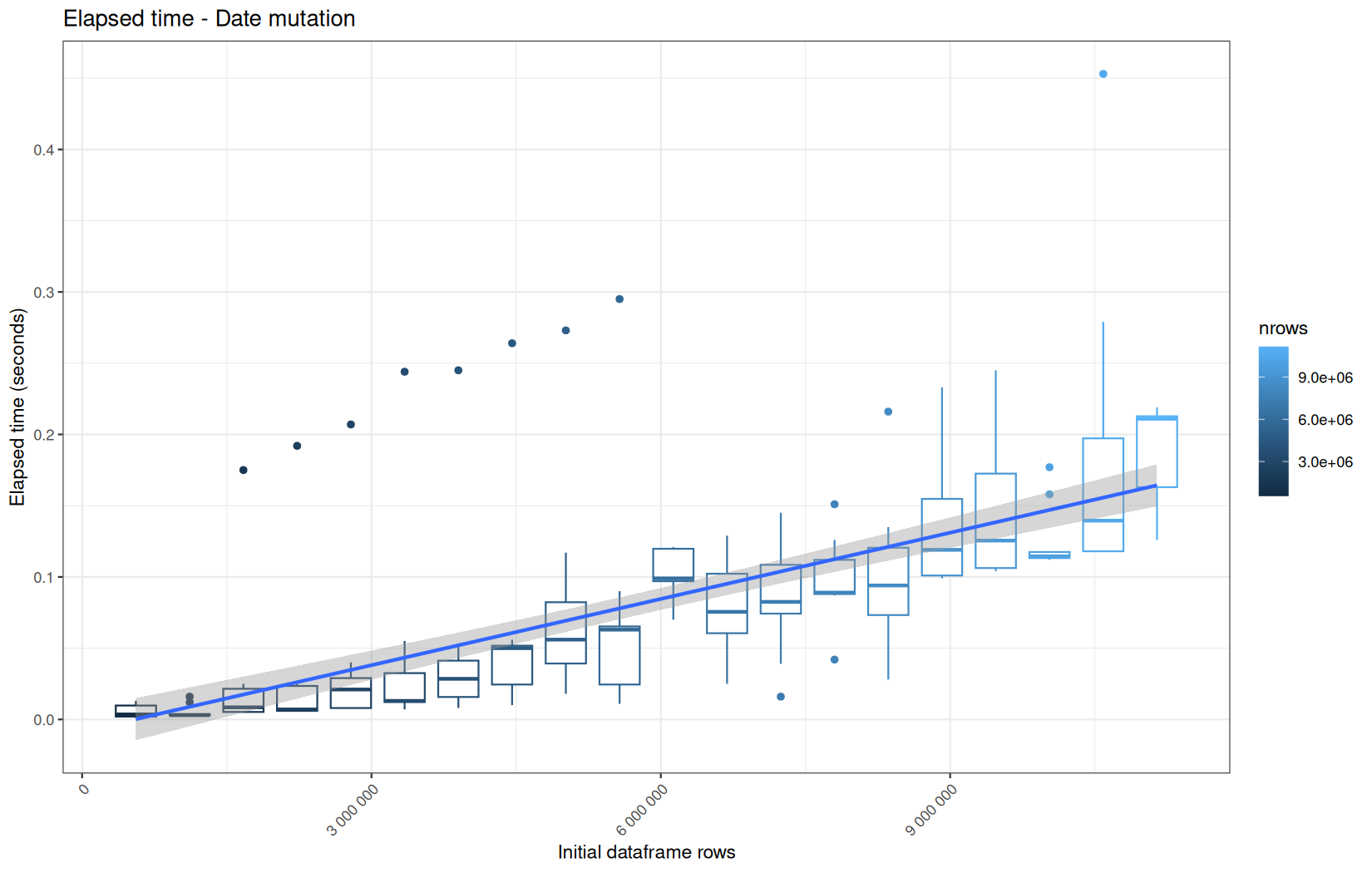
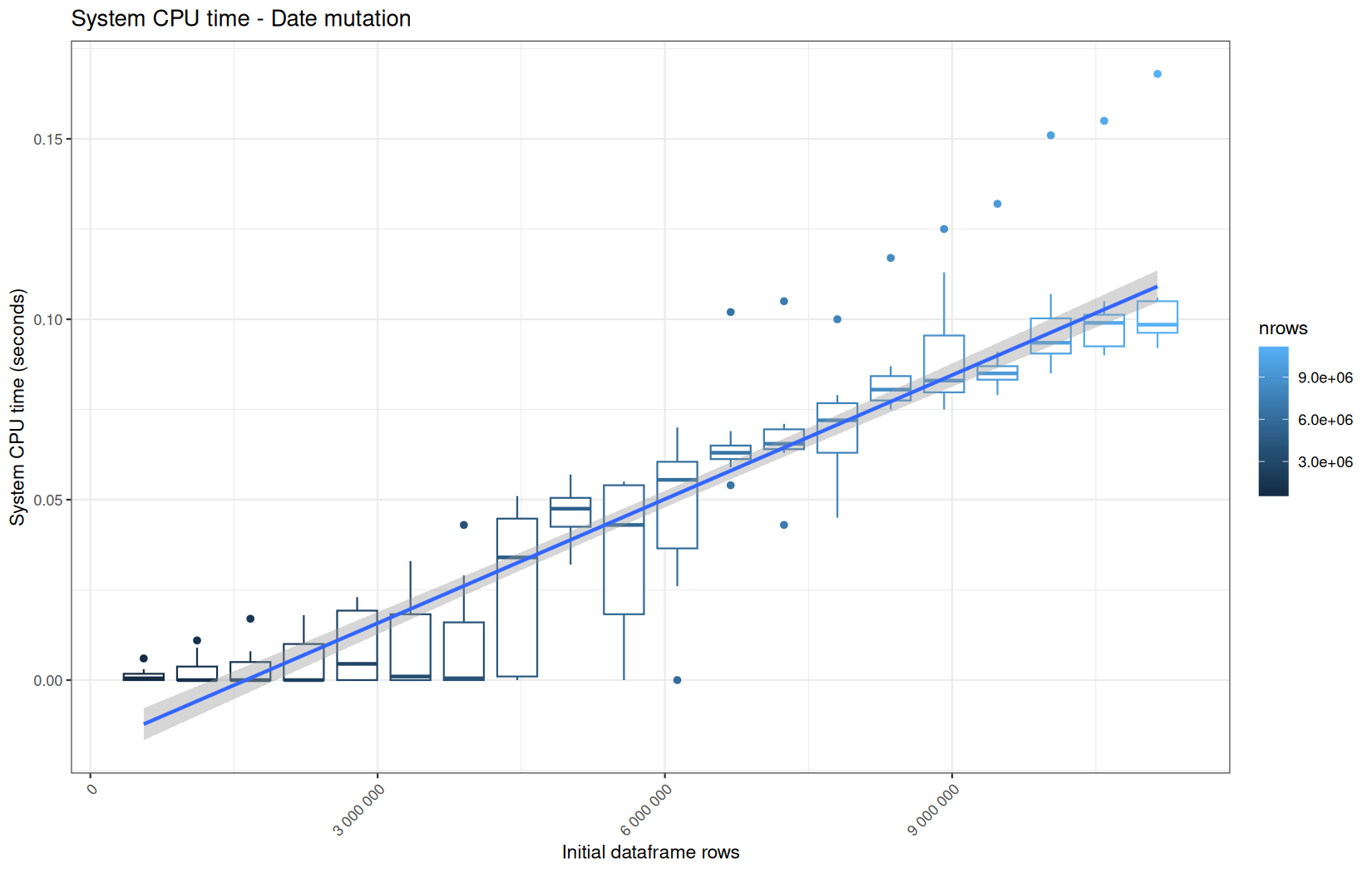
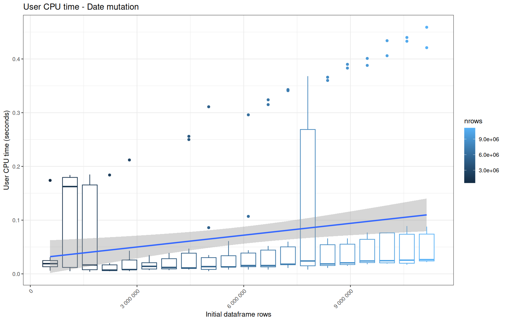
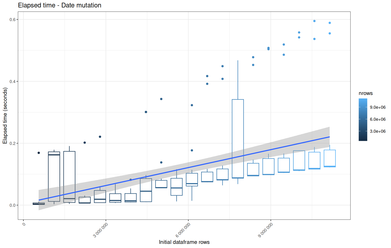
There is no surprise, all backends perform on the same level, and cold-start are linearly above the median.
But, we see that the variance in the hot runs is higher than for the ingestion path.
Now, we will compare to dplyr.
dplyr
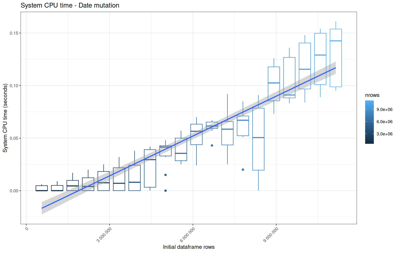
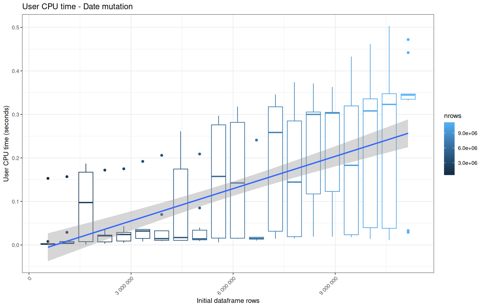
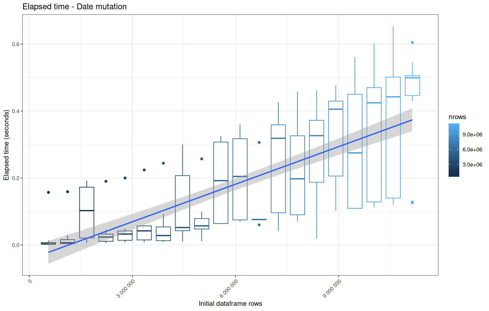
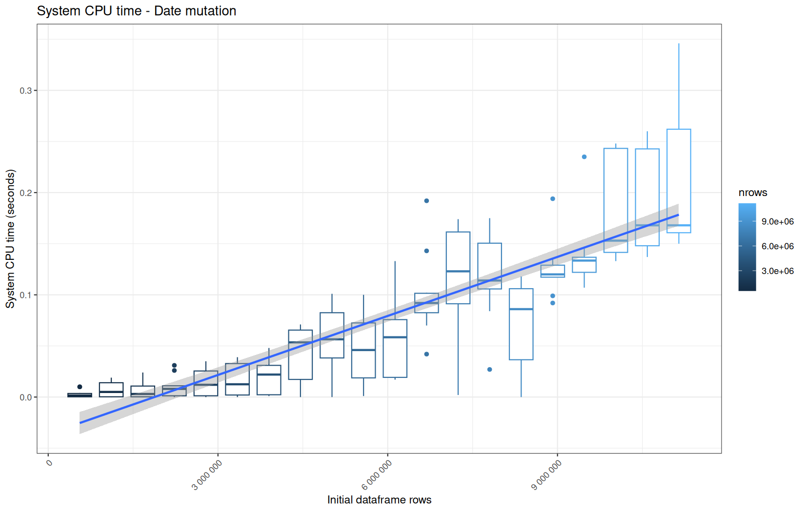
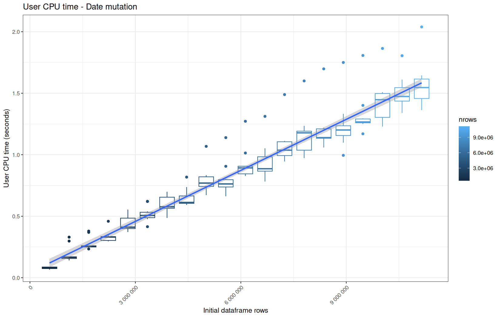
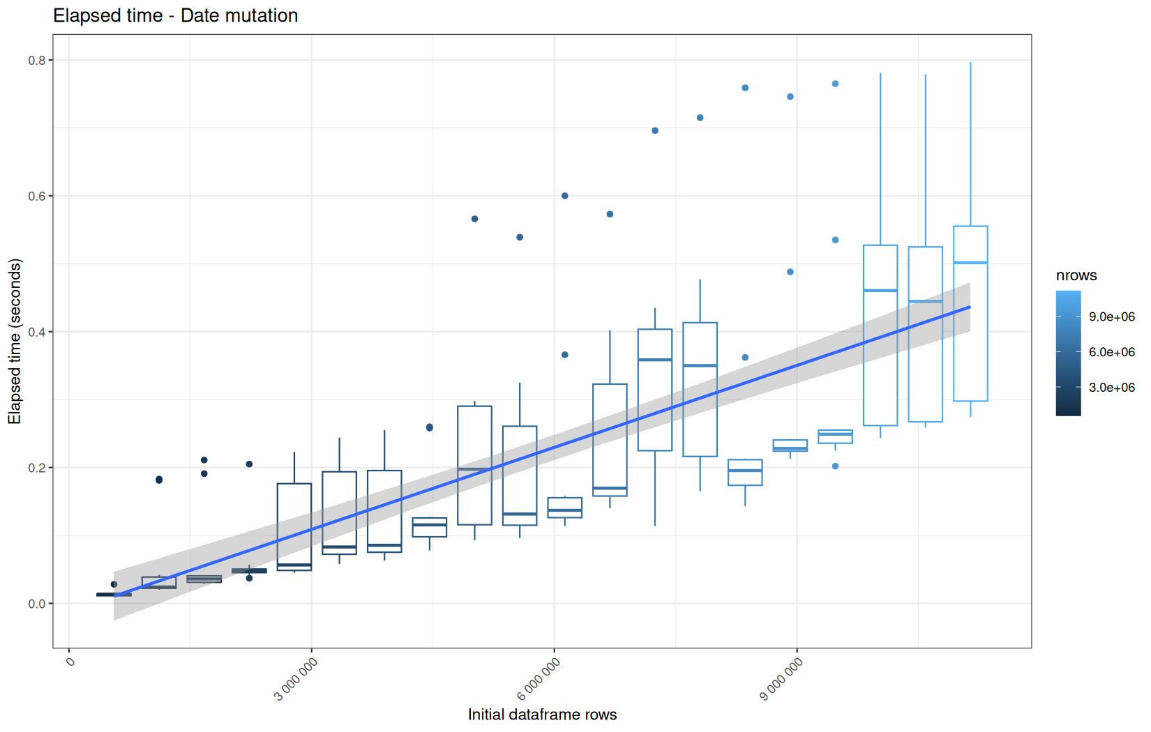
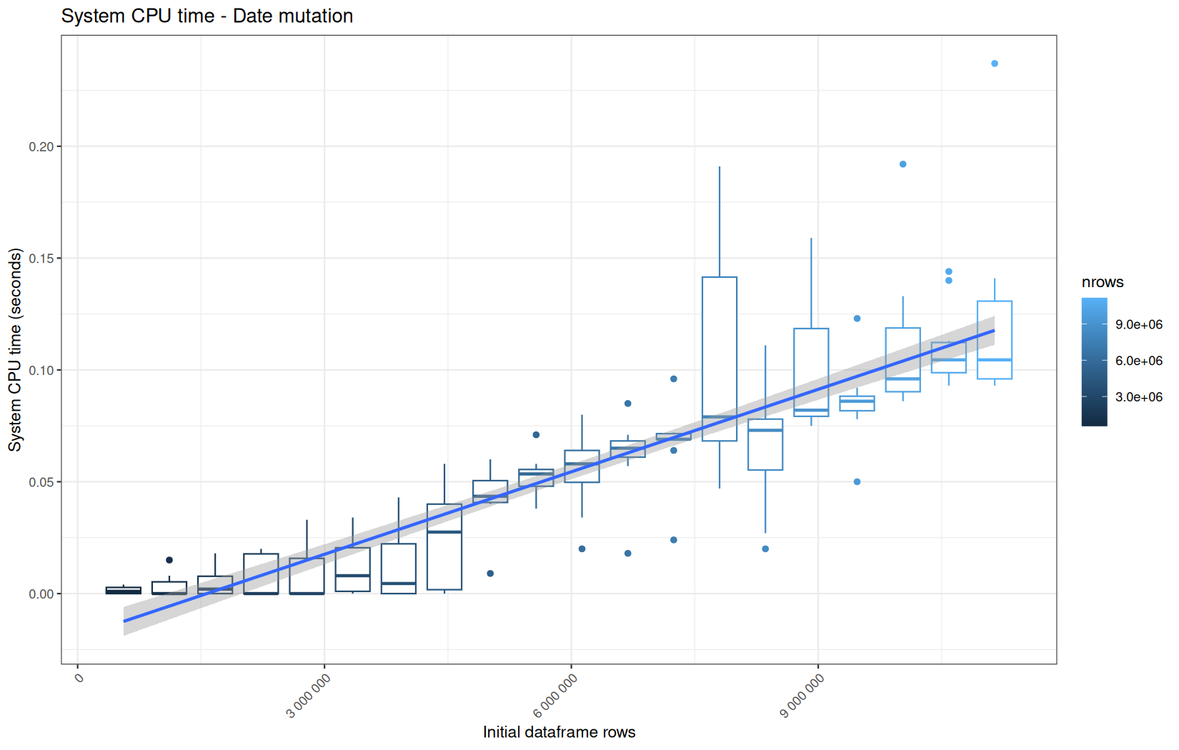
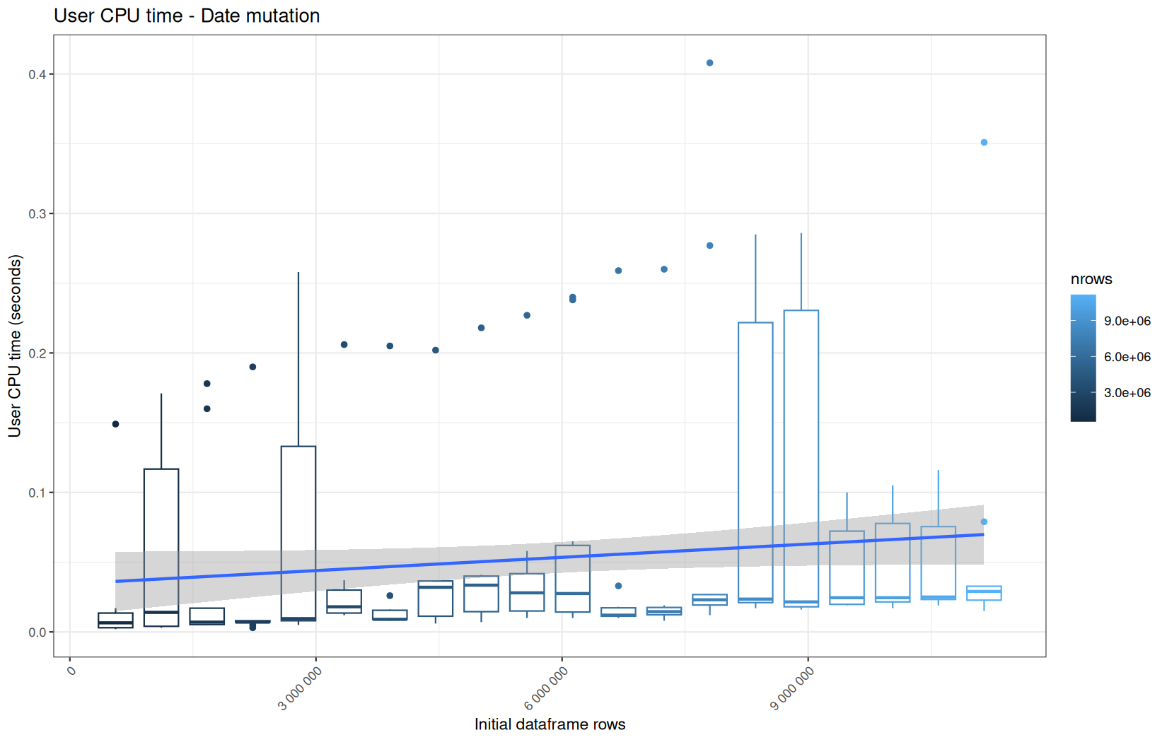
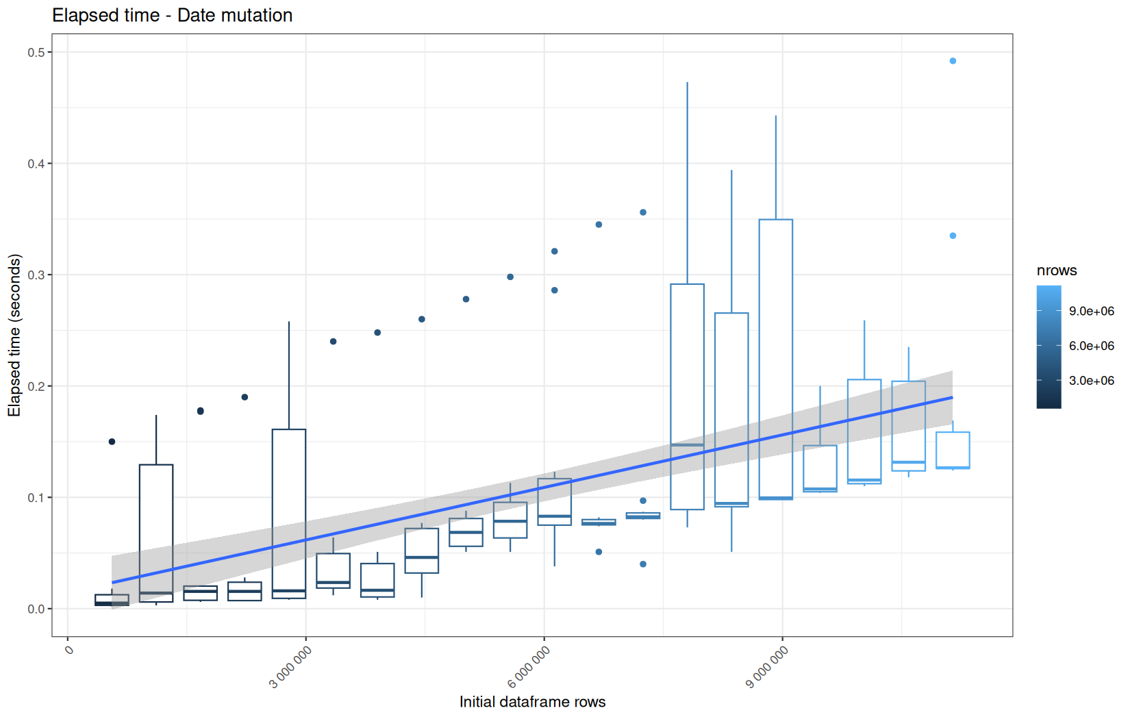
With no surprises, vroom path perform worst here because of the delayed materialization.
But its results are no too far away from readr path, and why does readr path is noticeably slower than the fread path while at this moment they are both tibble and the same dplyr operation is applied ?
Ok, after some searches, I found out that tibble is a very general container, meaning that a some metadata can be attached to certain variants.
In this case, especialy readr tibble flavor has a special tibble variant called spec_tbl_df.
We can confirm this by running the following code on the dataframe:
print(class(df))
print(names(attributes(df)))
The first wil tell the class hierarchy of the object and the second wil show you all the attributes attached to the object.
For fread -> tibble we got:
[1] "tbl_df" "tbl" "data.frame"
[1] "row.names" "names" "class"
Meaning that the dataframe returned by this path is a tibble, we see it reading those tbl (general tibble class) and tbl_df (concrete tibble dataframe).
And it has 3 attributes which are common and minimal such as names, class and row.names.
But, looking at what readr -> tibble path is providing, this is not the same story.
[1] "spec_tbl_df" "tbl_df" "tbl" "data.frame"
[1] "row.names" "spec" "problems" "names" "class"
Yess, the tibble-readr flavor named spec_tbl_df provides 2 other attributes:
spec-> stores the colupn type parsing specifications
Example:
attr(df, "spec")
Results:
cols(
ip = col_character(),
ts = col_double(),
target = col_character(),
status = col_integer(),
ua = col_character()
)
Its size is:
print(lobstr::obj_size(readr::spec(df)))
Result:
2.69 kB
So not really heavy, its raw size is not the root cause of the speed issue.
problems-> stores parsing issue, great for debuability
In fact this is a tibble that we can inspect like:
print(readr::problems(df))
In this case it is empty because no issues:
# A tibble: 0 × 5
# ℹ 5 variables: row <int>, col <int>, expected <chr>, actual <chr>, file <chr>
Its size as an empty 5 columns tibble is also not large:
print(lobstr::obj_size(readr::problems(df)))
1.36 kB
But, when dplyr mutates the object, it has to reconstruct the output while preserving the relevant attributes and class structure of the input.
Therefore, the spec_tbl_df class and its spec / problems attributes may participate in the reconstruction path, even if the mutation itself only touches the ts column.
This can create a small but measurable overhead compared with a plain tibble coming from fread -> as_tibble().
The small overhead is not due to the problems size tibble but rather to:
extra method dispatch + attribute handling + reconstruction logic
Now, what the memory consumption tell ?
memory consumption
data.table
Current NCells:
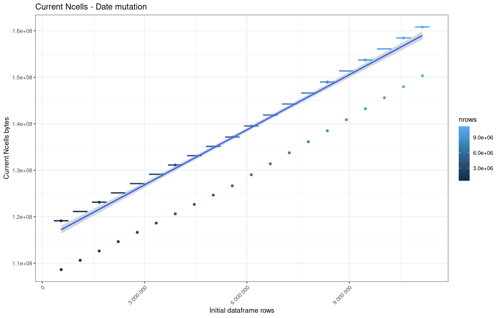
Current VCells:
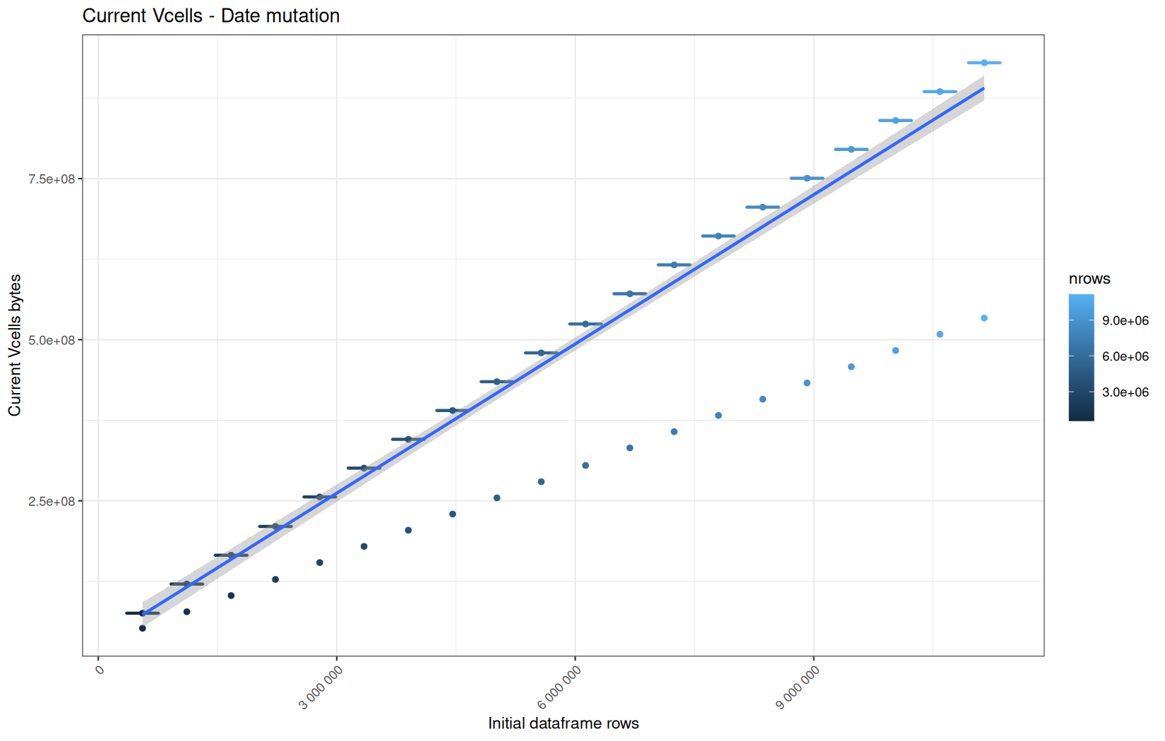
Max NCells:
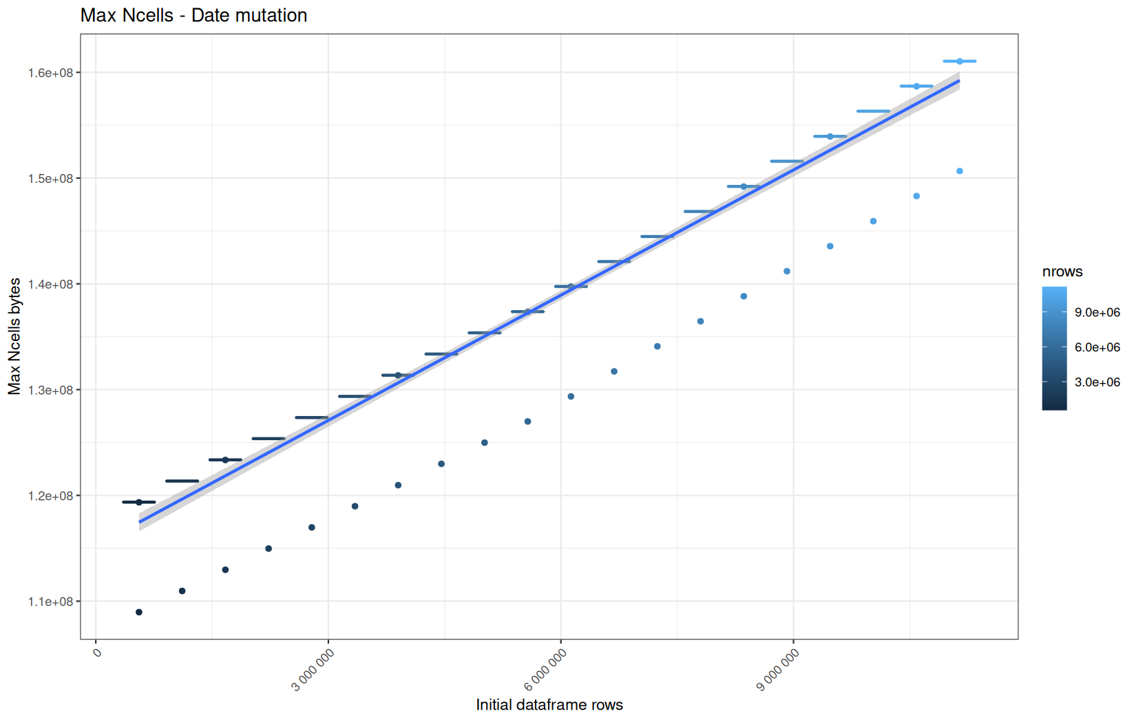
Max VCells:
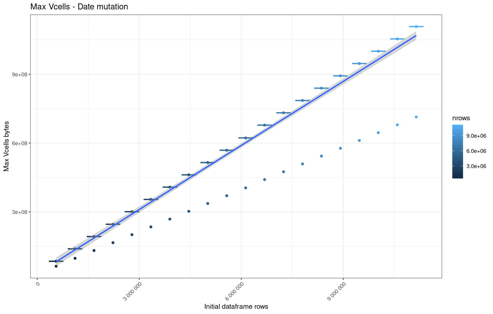
Current NCells:

Current VCells:

Max NCells:
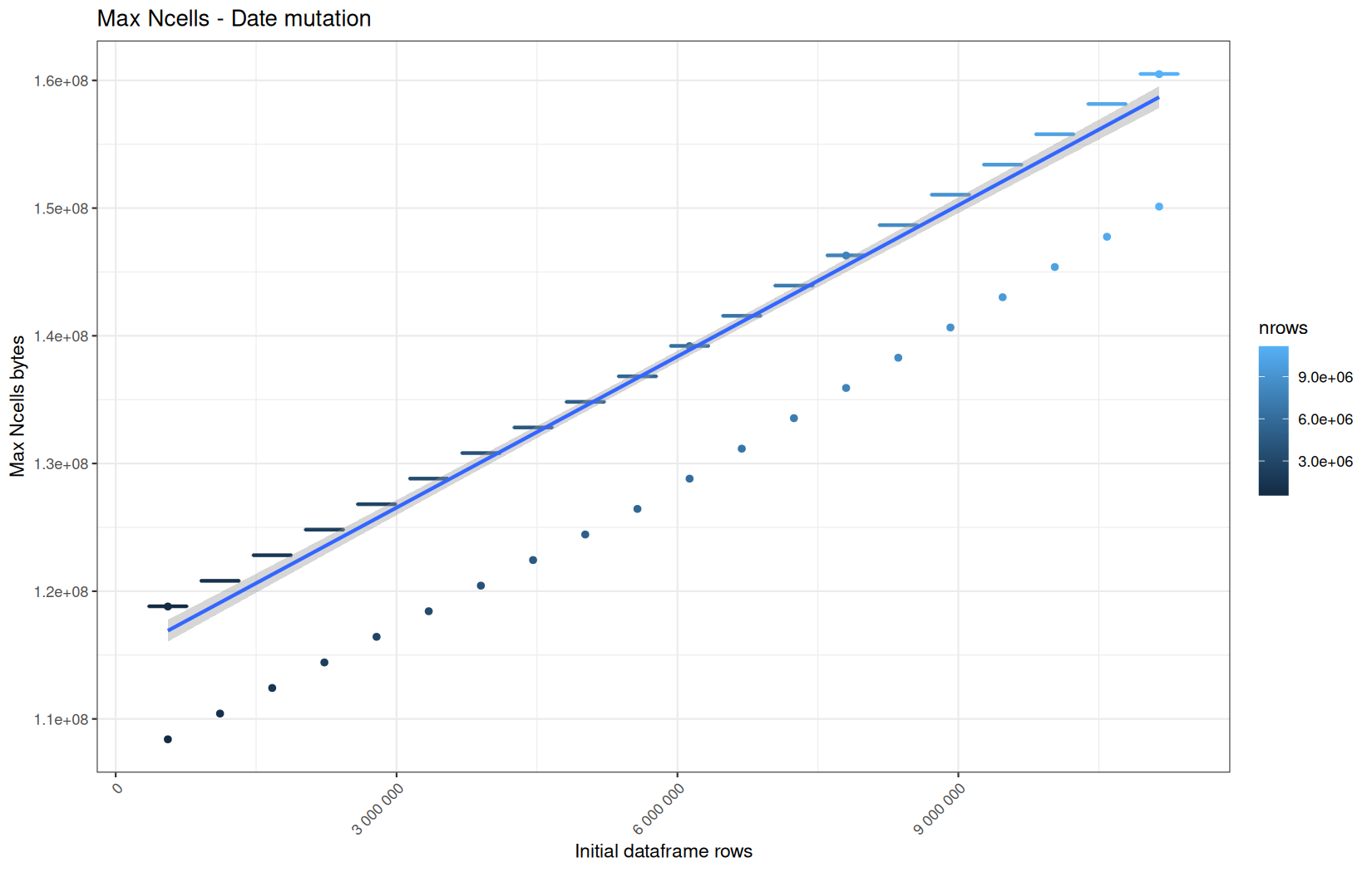
Max VCells:

Current NCells:
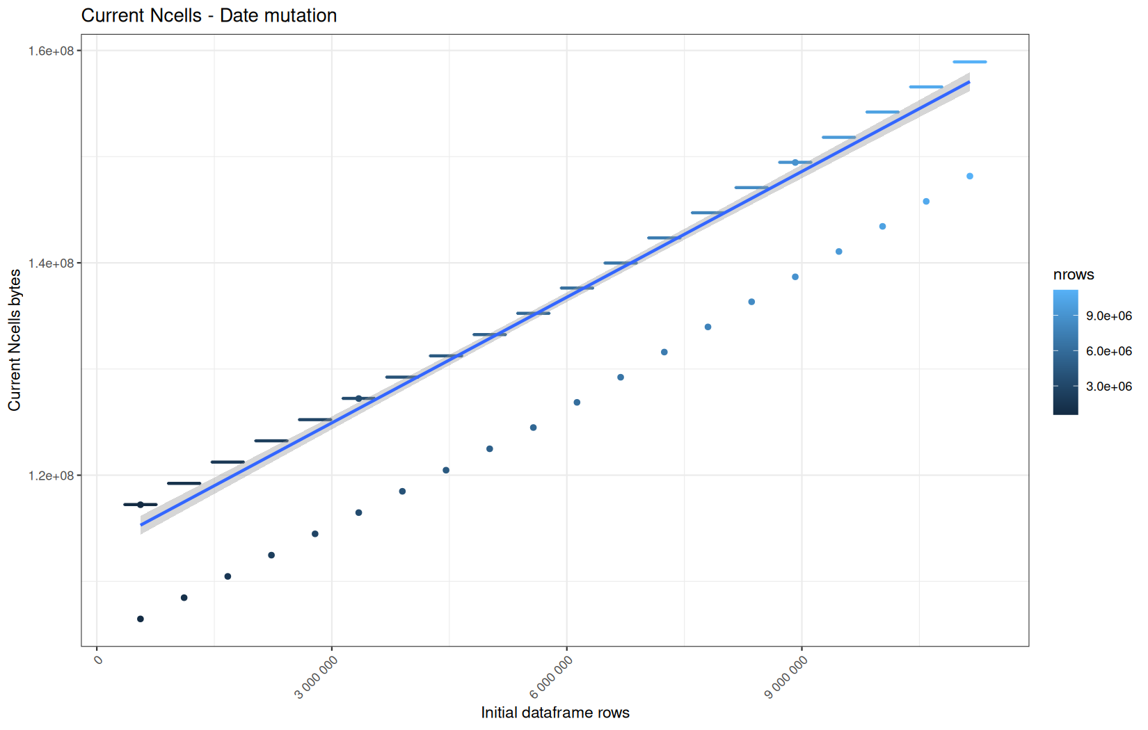
Current VCells:

Max NCells:
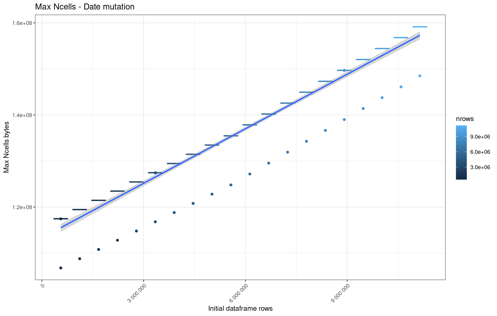
Max VCells:

Here, no surprises that the behaviour of readr and vroom path are the same.
But the real difference comes to current_vcells and max_vcells between fread and vroom/readr path.
We significantly use more VCells on the fread side.
I'm again surprised because at this point they are all sensed to be simple data.table and we apply the same operation so the same memory profile should be observed, but it is not the case.
This is simpler than before story, because all path lead to the same kind of data.table:
print(class(df))
print(names(attributes(df)))
Results:
[1] "data.table" "data.frame"
[1] "names" "row.names" "class"
[4] ".internal.selfref"
Rememeber, because the previous data.table operation with fread which was just the ingestion consumed more memory, so even after a garbage collection cycle, there are still more reachable R elements so the baseline is higher.
Hence from this point we are not able to identify a specific memory profile for the next operations, even analyzing only the cold start because already polluted by before operations.
But we can still see how the memory consumption of the pipeline evolve.
For the rest of the article, I will avoid interpreting memory usage as a strict per-operation allocation profile. I will use it mainly to describe the evolution of the whole pipeline and the effect of warm R-process state.
Anyway, here is the link of the files containing all the plots if you want (zip) :
dplyr
Current NCells:

Current VCells:

Max NCells:

Max VCells:

Current NCells:
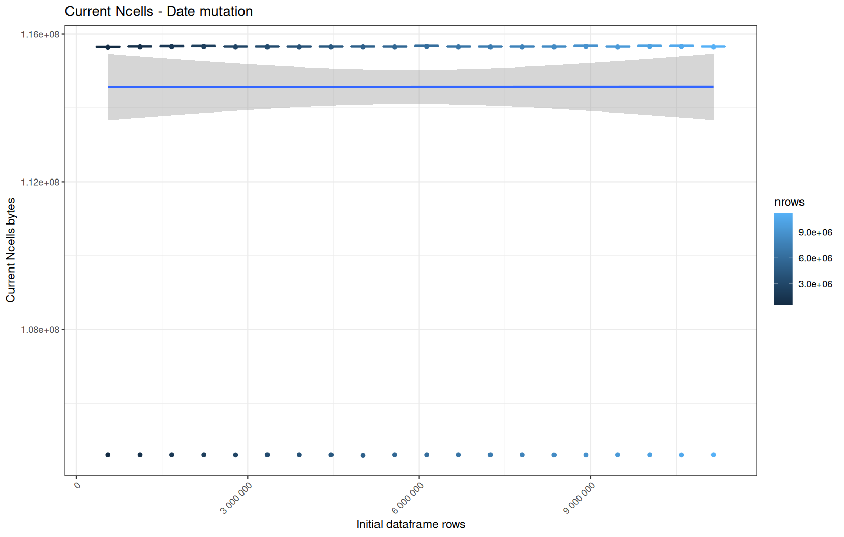
Current VCells:
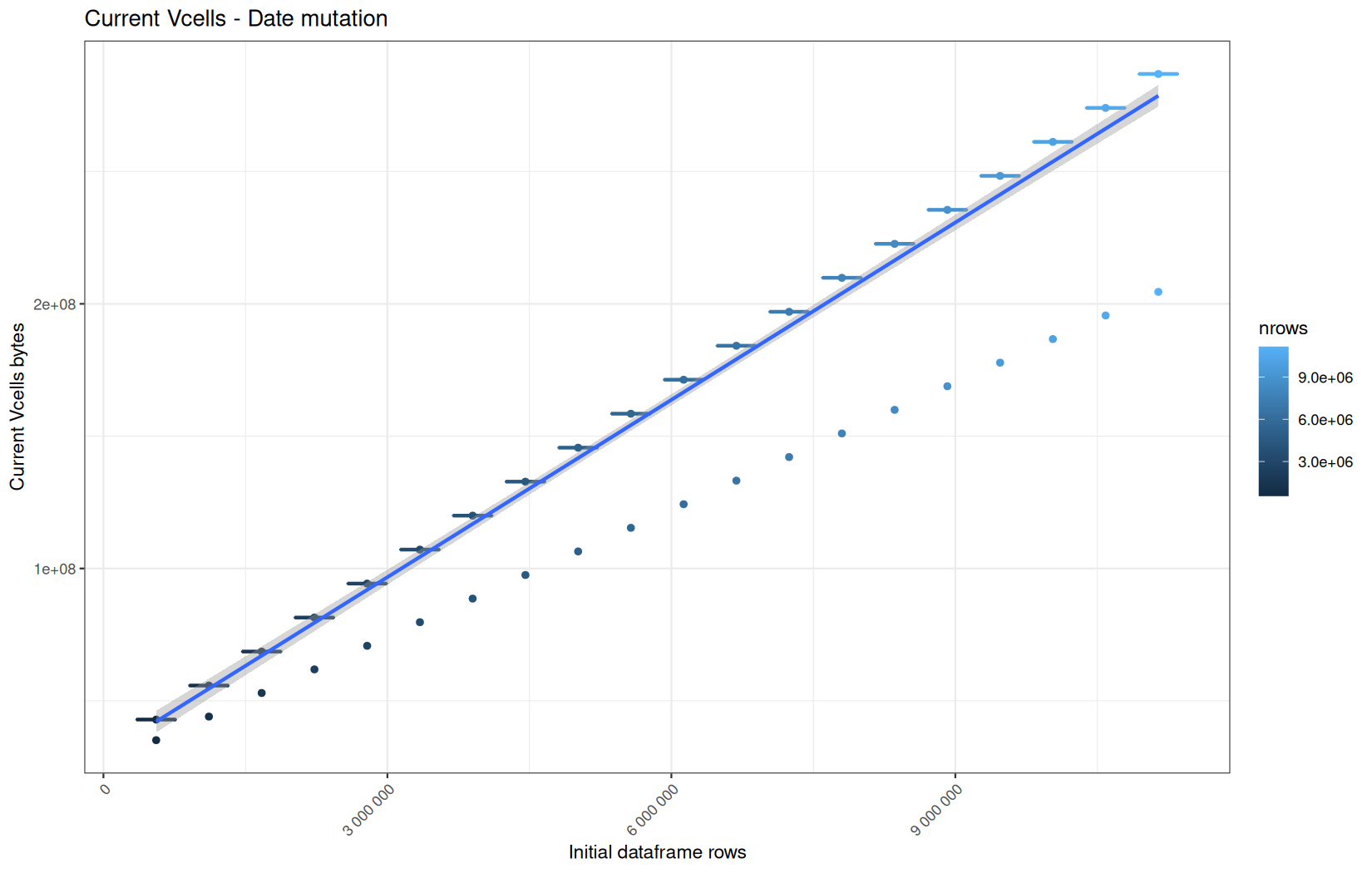
Max NCells:
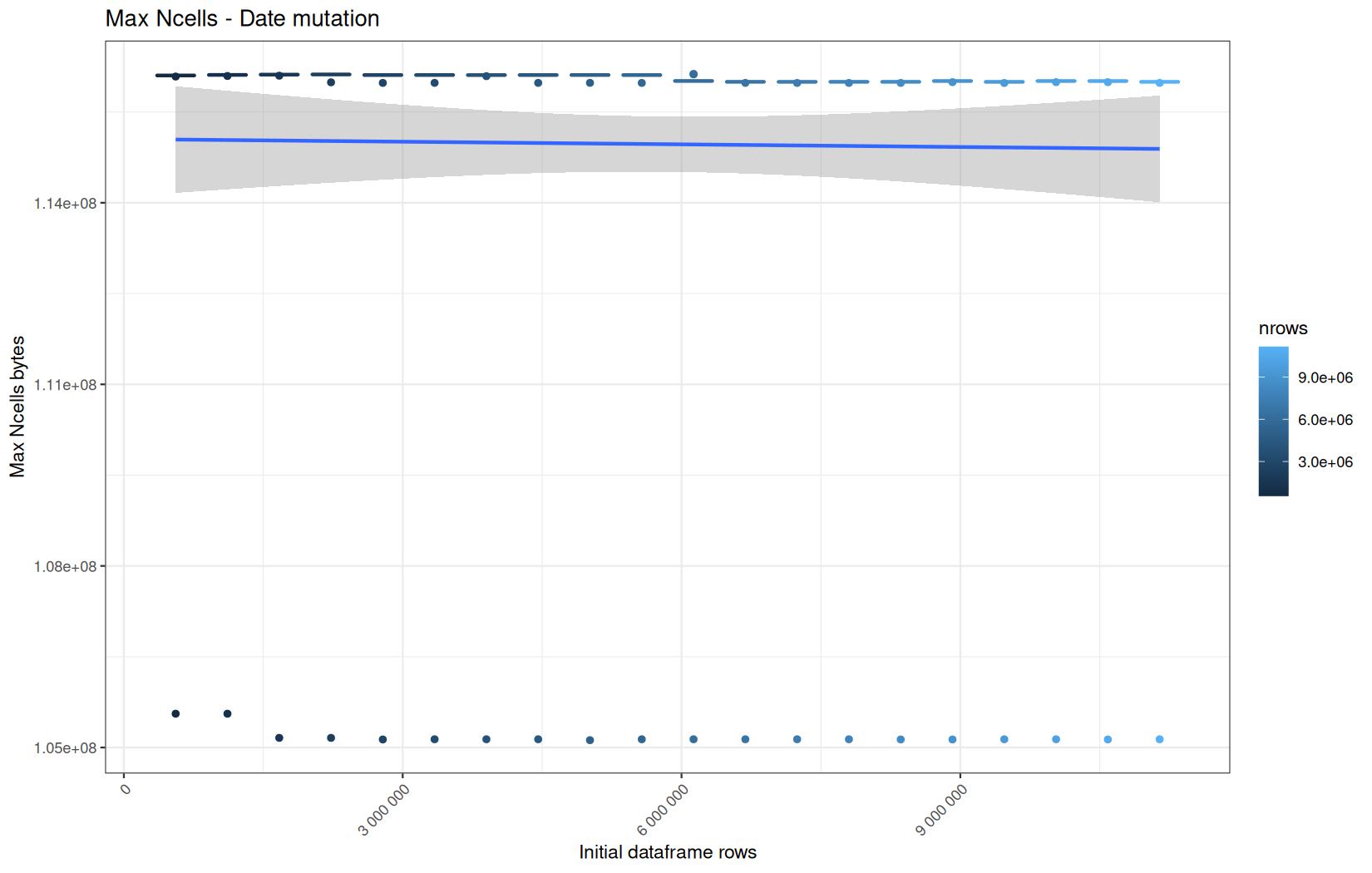
Max VCells:
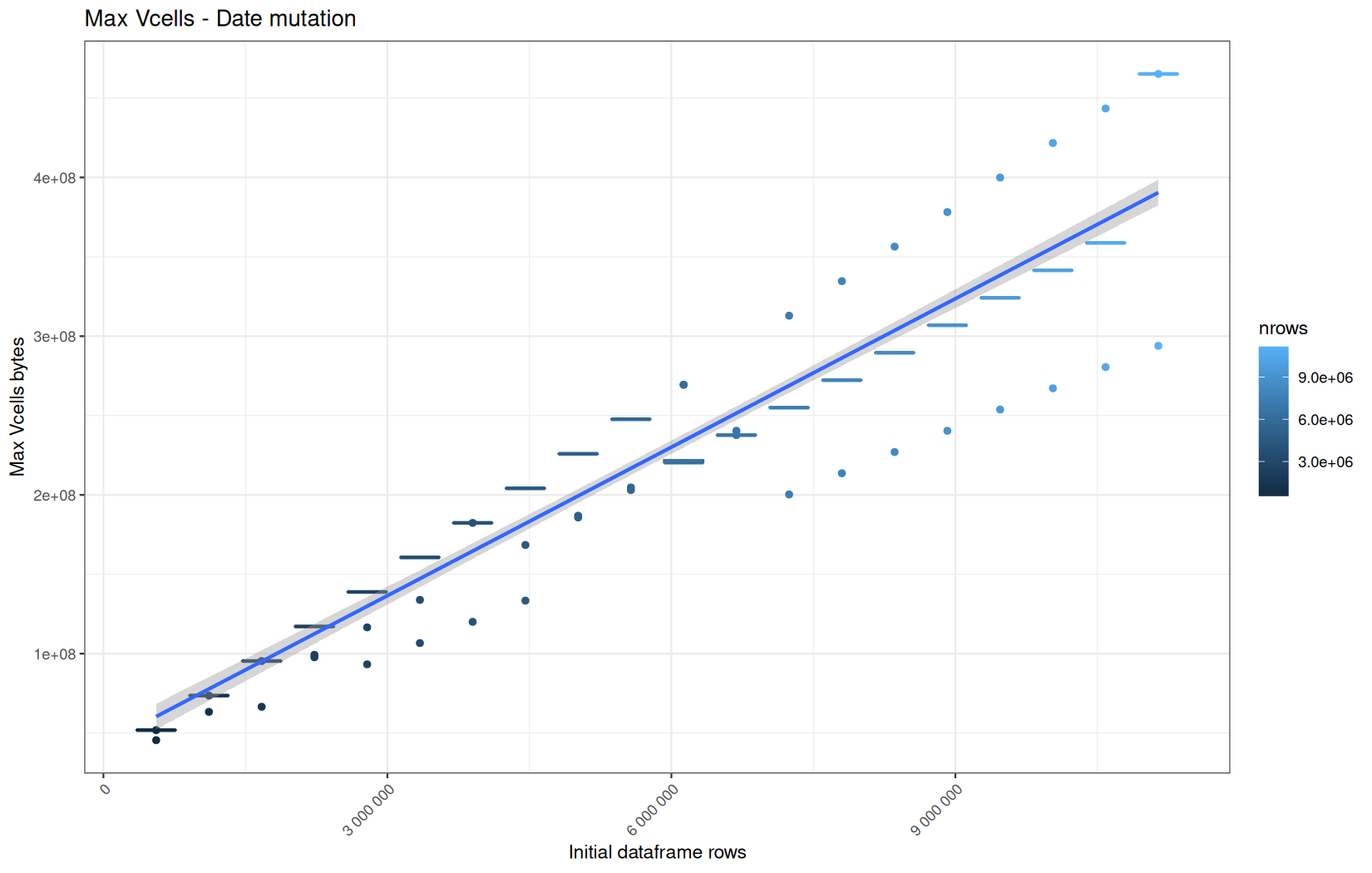
Current NCells:

Current VCells:
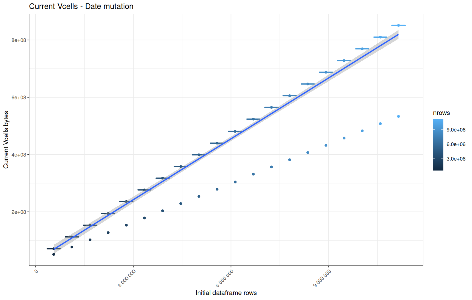
Max NCells:
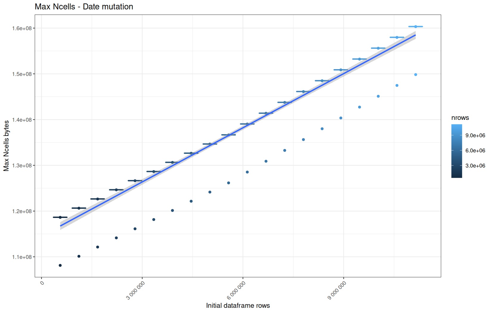
Max VCells:

The readr + data.table and readr + dplyr path roughly have the same profile which is expected.
And the fread + data.table have higher VCells values than fread + dplyr which is expected because of the hiher memory baseline in the data.table path like explanined before.
It become harder to realize a per-operation profile because of the pollution.
But we can still confirm that the materialization on vroom + dplyr happen in the targeted column (here date), because at this point the pipeline for this path consumes approximately 2 / 5 of the VCells memory compared to the readr + dplyr path, which is expected because only 1 out of 5 columns are materialized.
And yet again, the memory consumption of the vroom path remains stable for NCells.
If we zoom-out and look at all the max_ncells and current_ncells for this path, we see that all are constant.
The operations are not creating more R objects as the file gets larger.
And because NCells mostly represent R-level objects: lists, pairlists, attributes, symbols, metadata structures etc and that the files and later the tibble alsways have the same amount of columns, it suggest that NCells is not correlated to the number of rows but can be correlated to the number of columns.
We also observe the same cold-start outlier profile as in the ingestion process for the current_ncells cold-start being lower than the median.
But we can also note that it's also the case for the max_ncells for all data-manipulation operations which is the opposite of what hapened in the data-ingestion process where cold-start were above the median potentialy due to ingestion backend initialization.
One fun thing to note is that the constant values NCells are in the same order of magnitude of the NCells values of readr + dplyr and fread + dplyr.
This is potentially because the baseline for the R process is basicaly the same for all paths ( memory baseline pollution ).
From this point on, we will mainly focus on execution time, because the benchmark methodology gives us confidence that the per-operation results are reliable.
So now, for this operation and its dplyr equivalent:
data.table::setcolorder(df, c("ip", "ts", "target", "status", "ua"))
Execution time
data.table

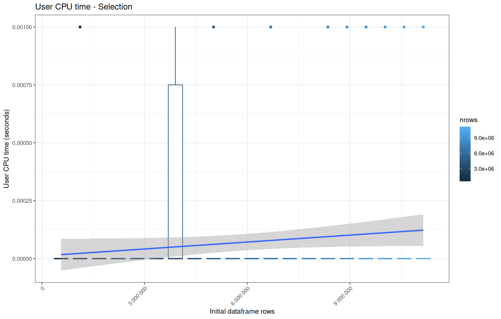
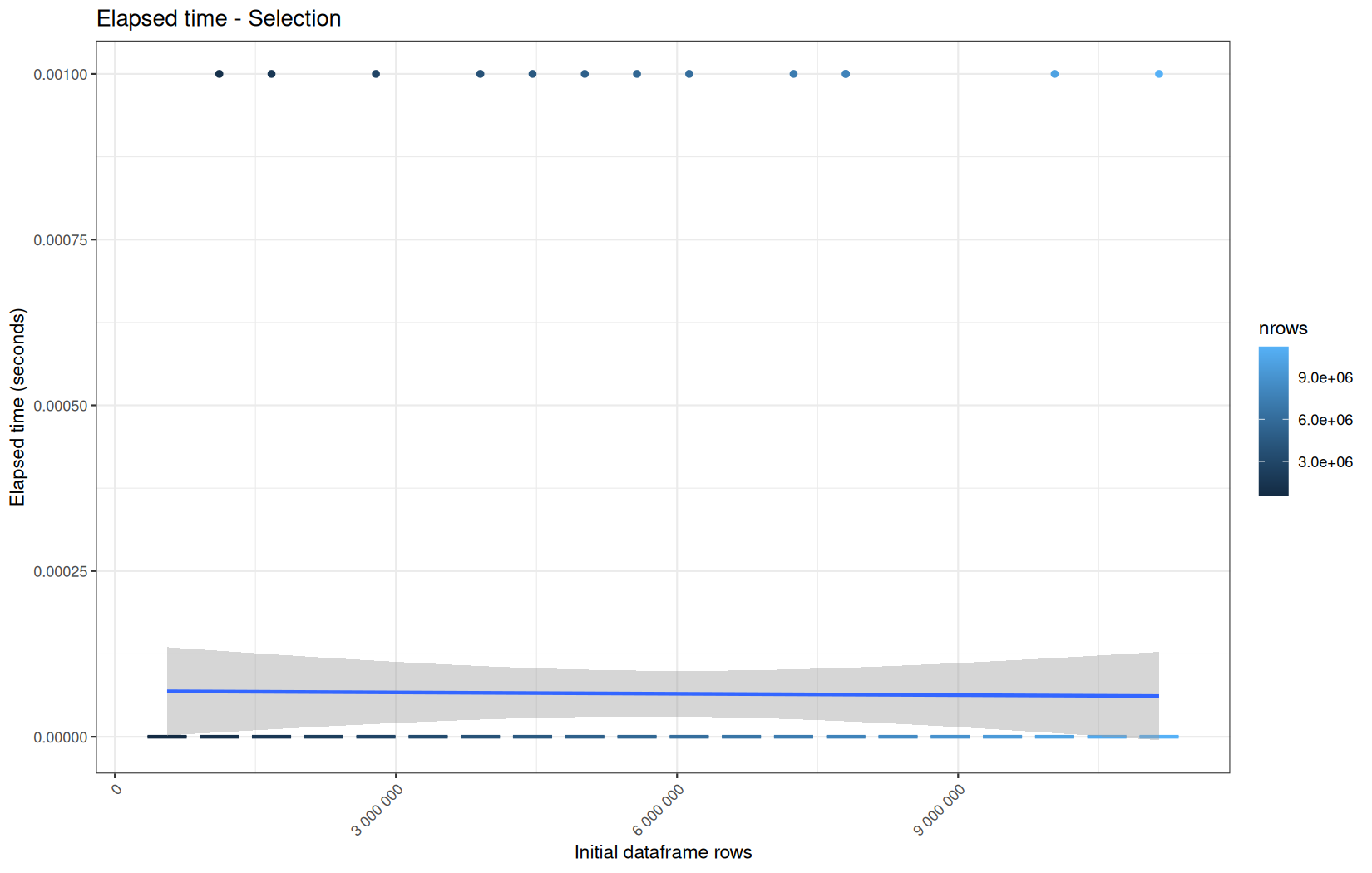
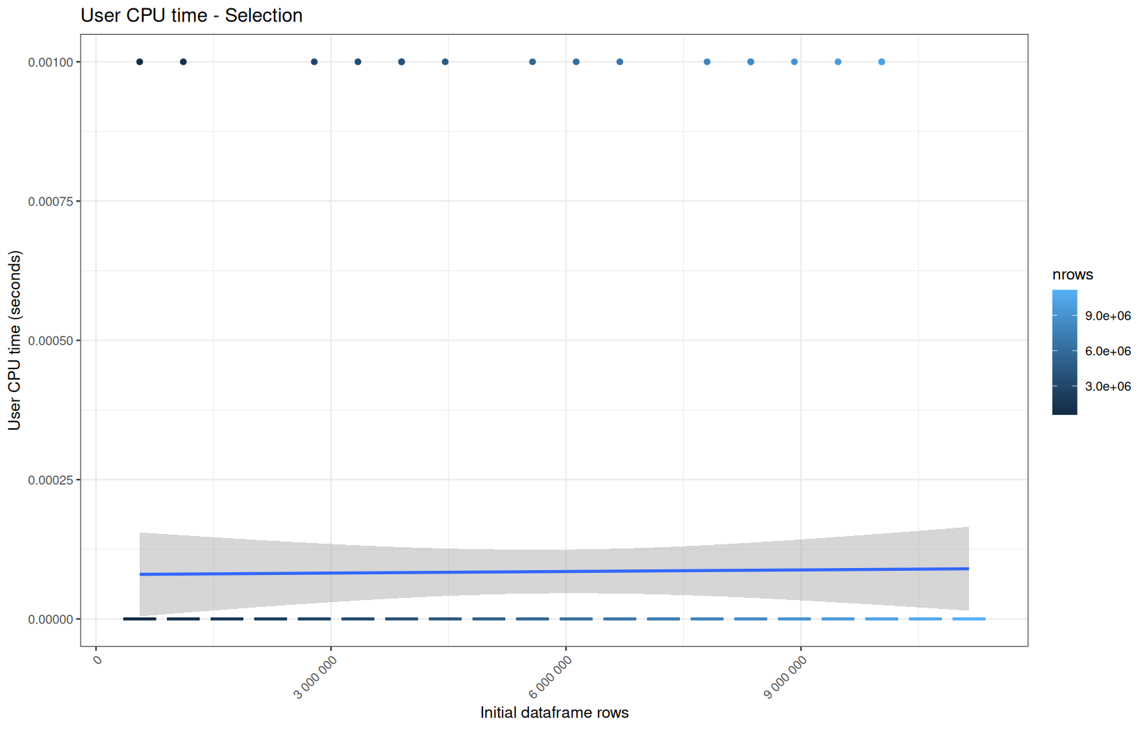
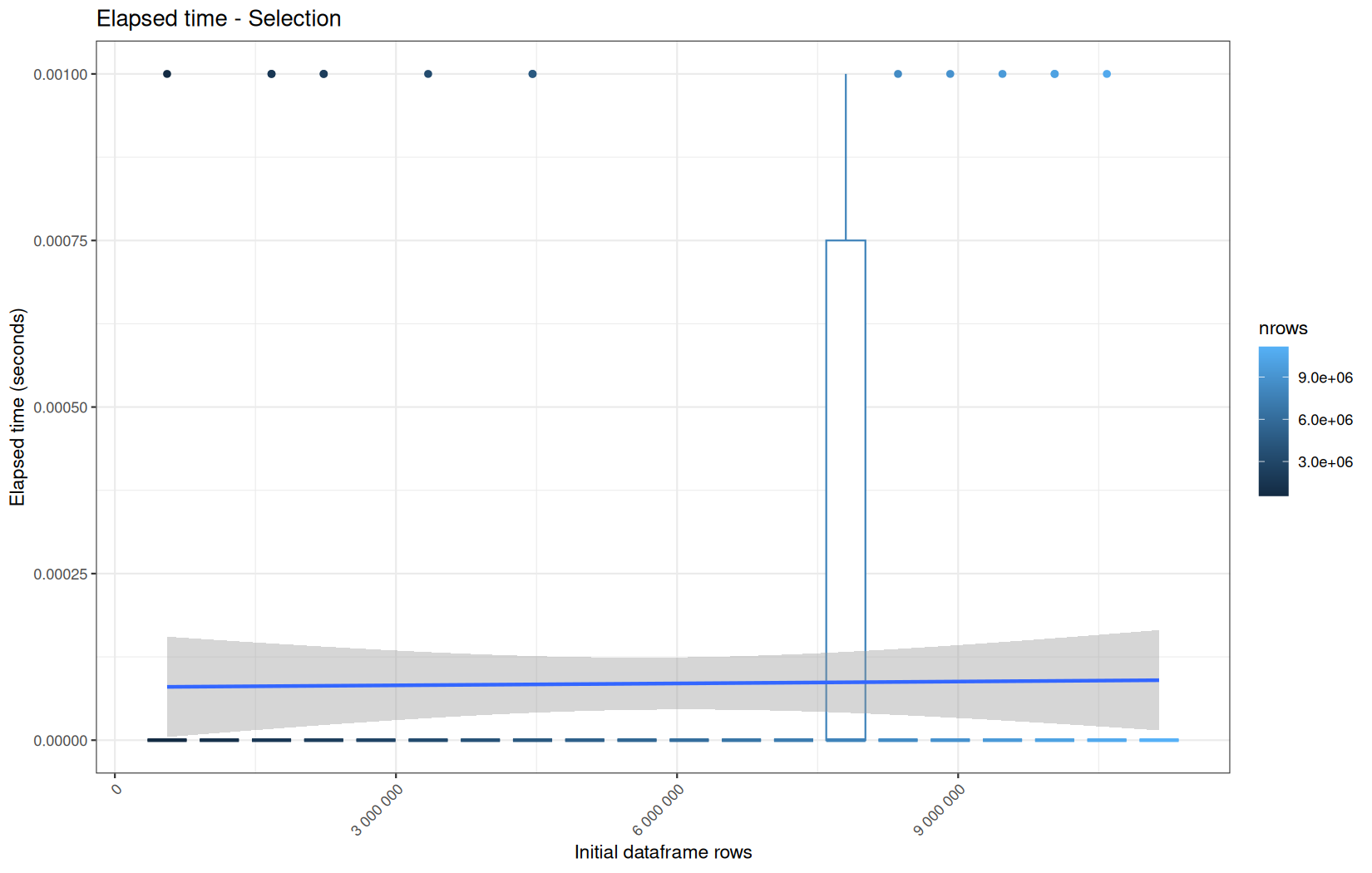

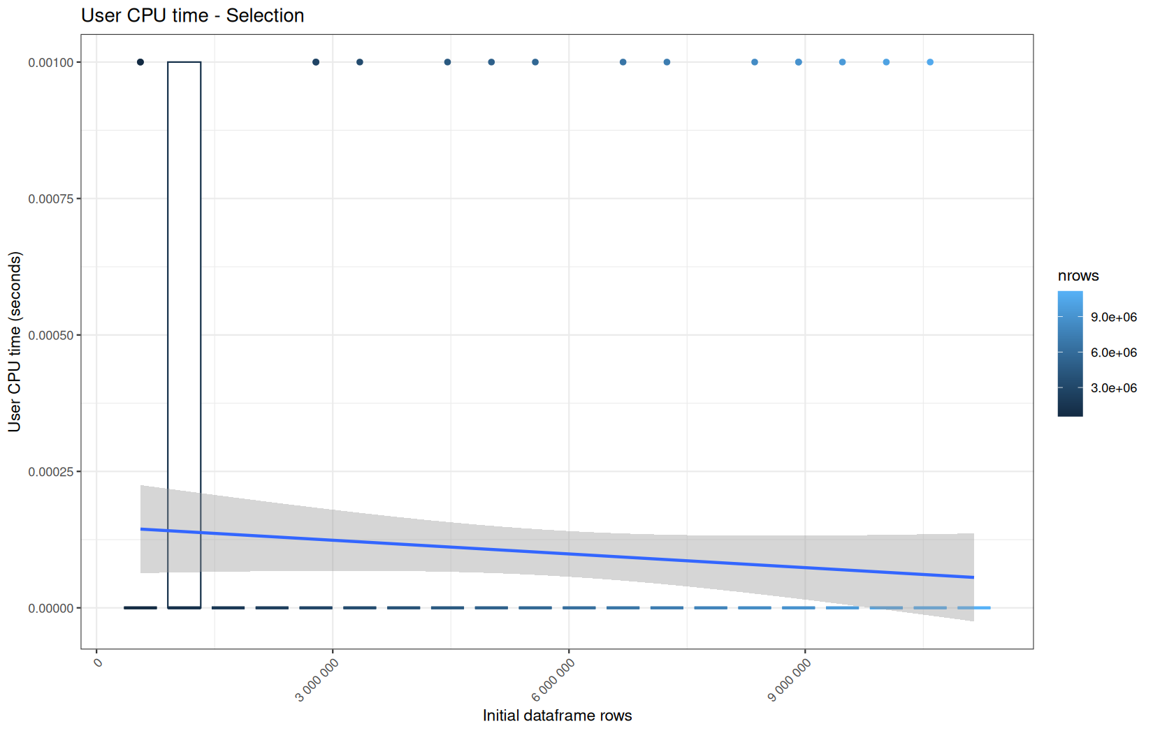
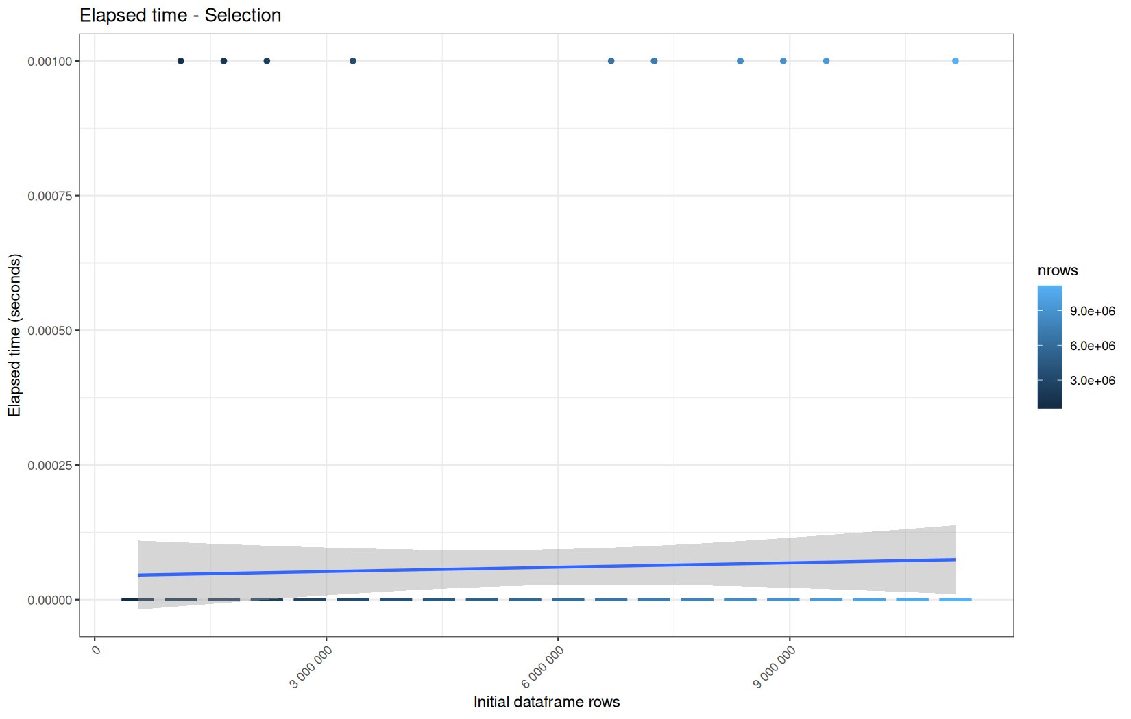
No surpises, all have roughly the same profile, the interresting thing is tom compare them to the dplyr variant.
dplyr
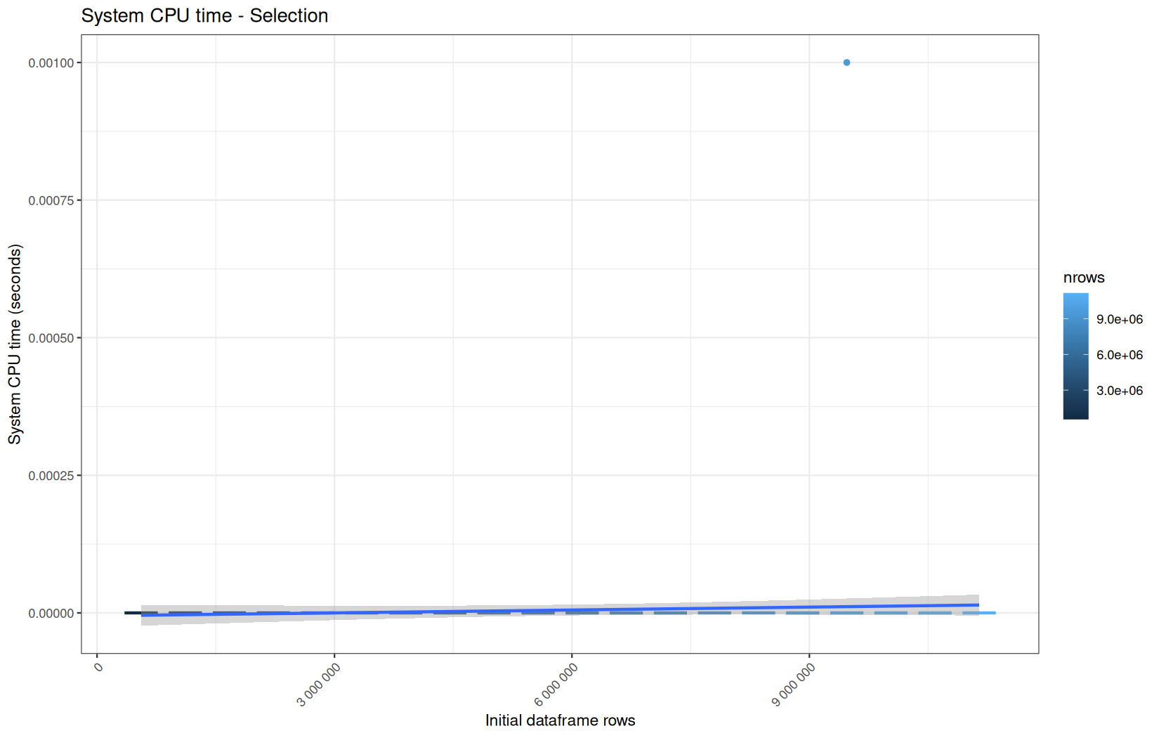
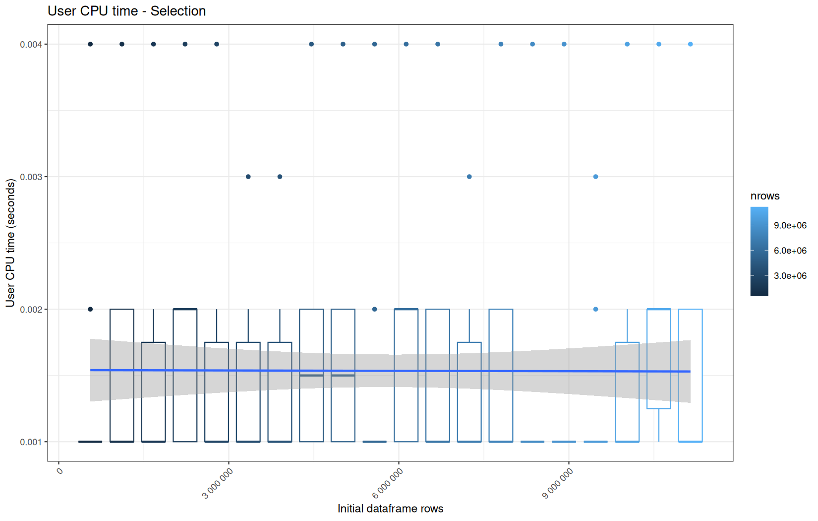
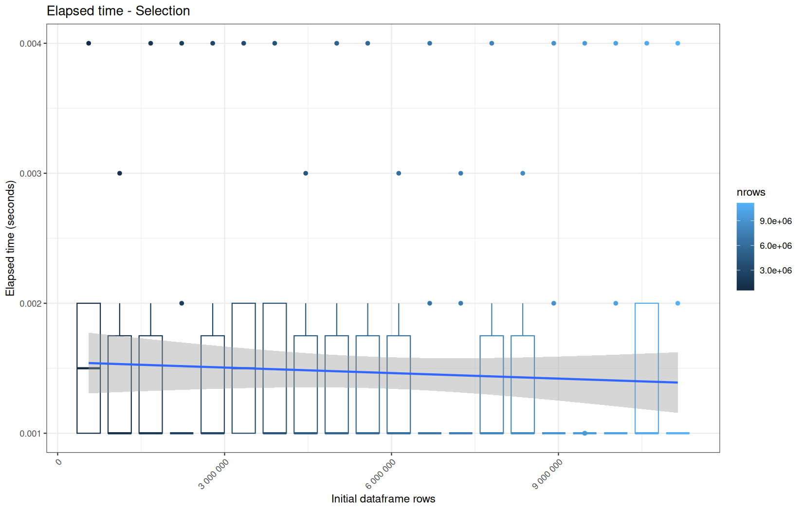
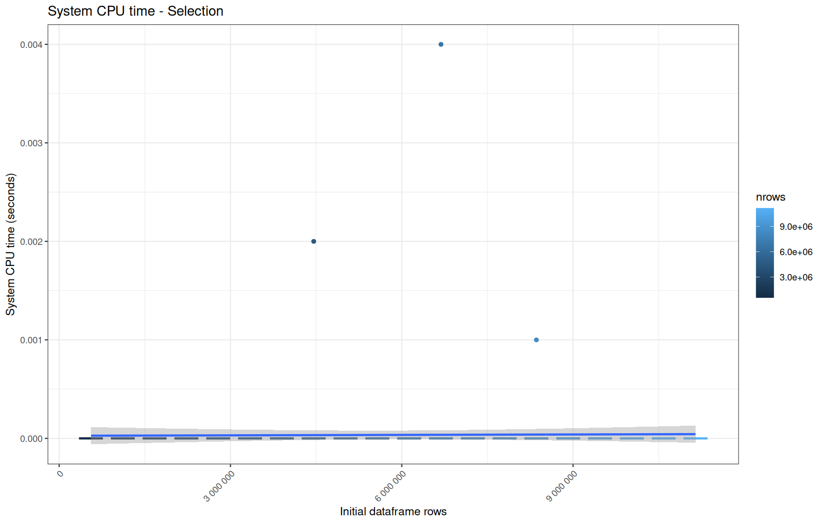

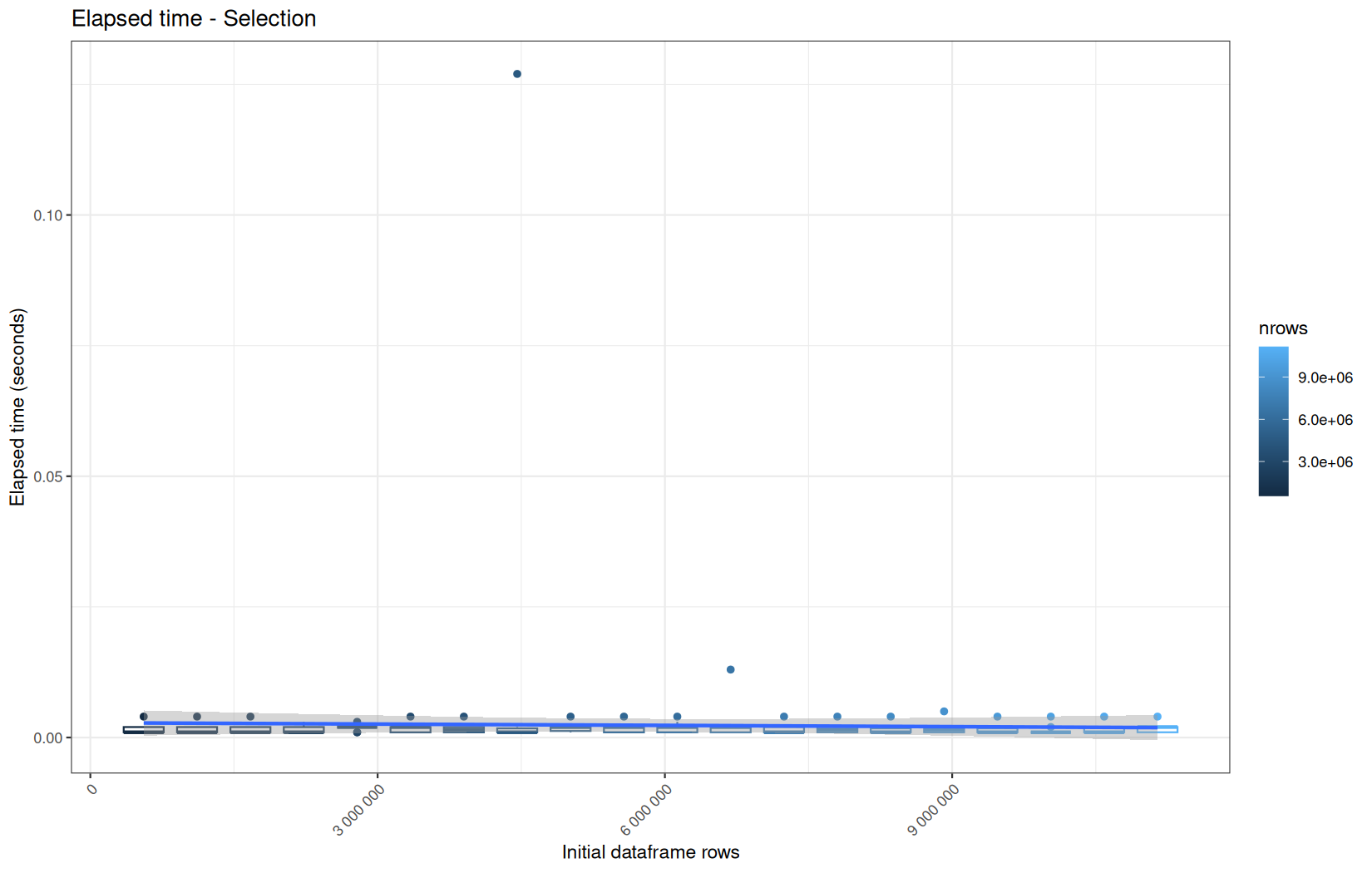
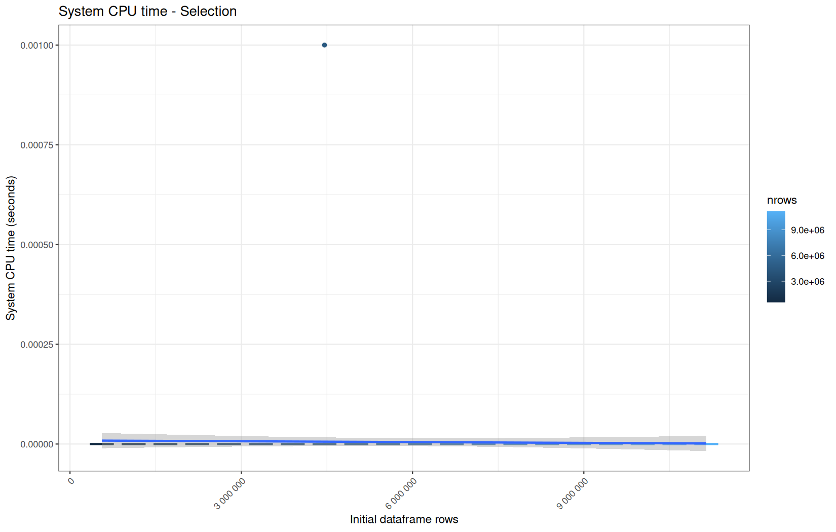
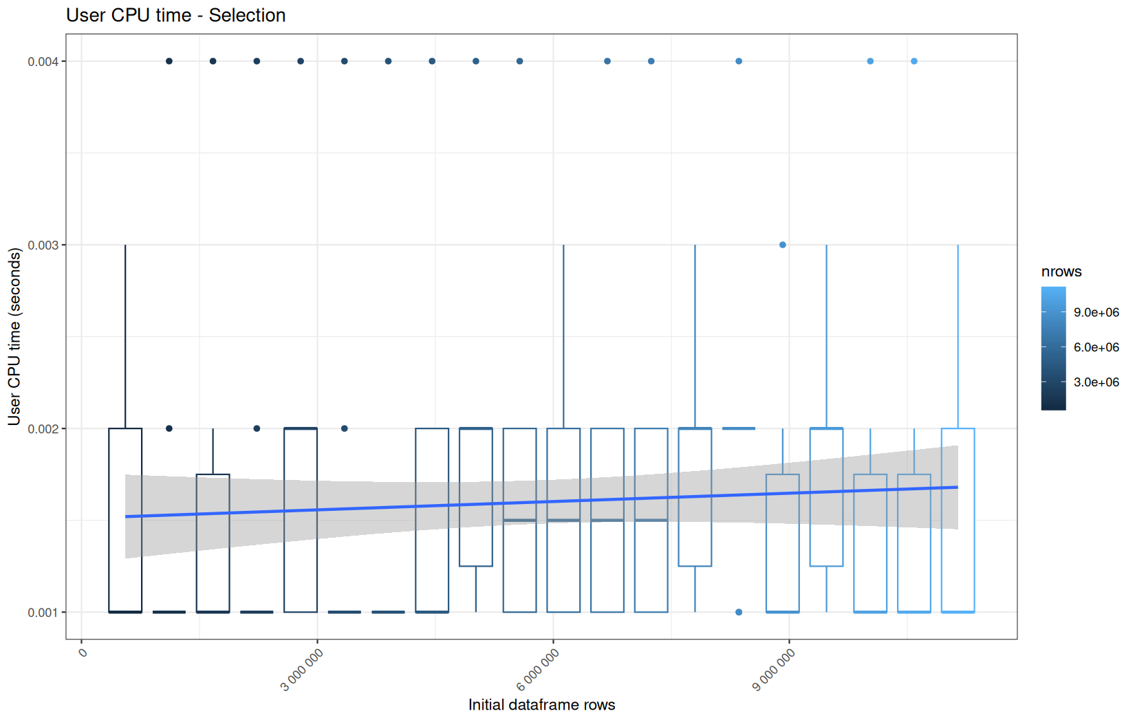
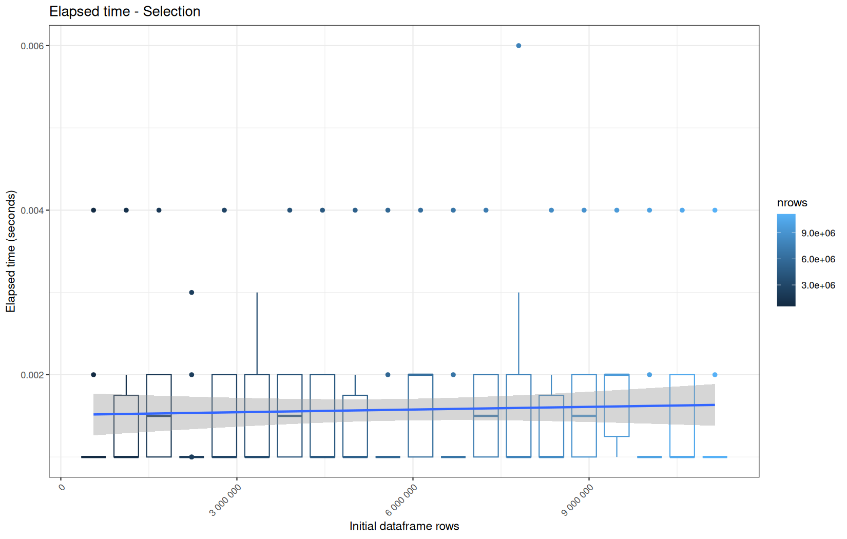
No surpises, also roughly the same profile.
And as expected, they are not multithreaded, like the data?.table variant.
But most importantly, they have a higher value of execution time than the data.table variant.
We explain why in the previous article. (because data.table operation is in-place and basically just do some pointers work while the dplyr variant must recosntruct a tibble container, but still not huge alloc for each one of the columns -> columns are shared).
Now we go ahead for this operation and its dplyr equivalent:
log_step("Filtering", {
df <- df[!is.na(date) &
!is.na(target) &
!is.na(status) &
status == 200]
})
Execution time
data.table

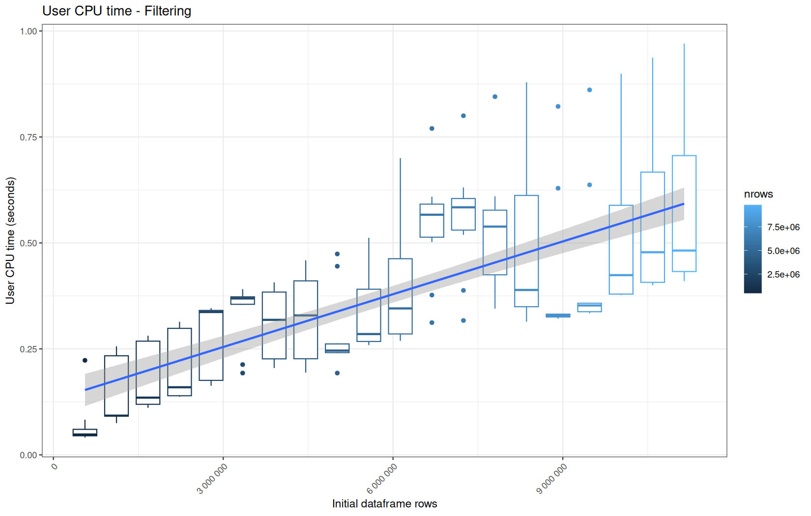
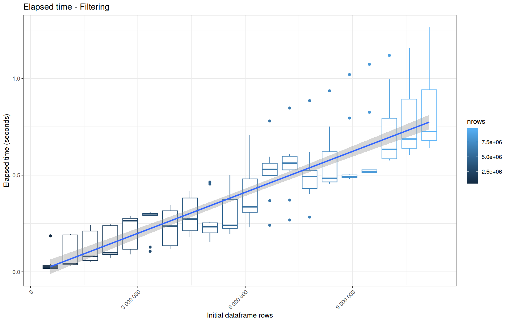
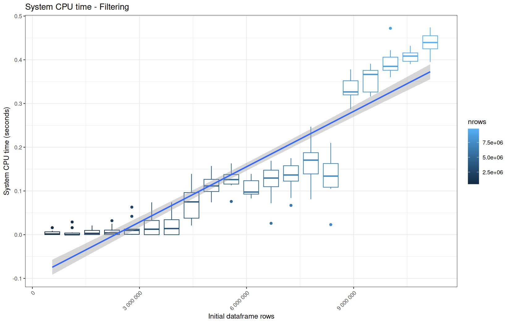
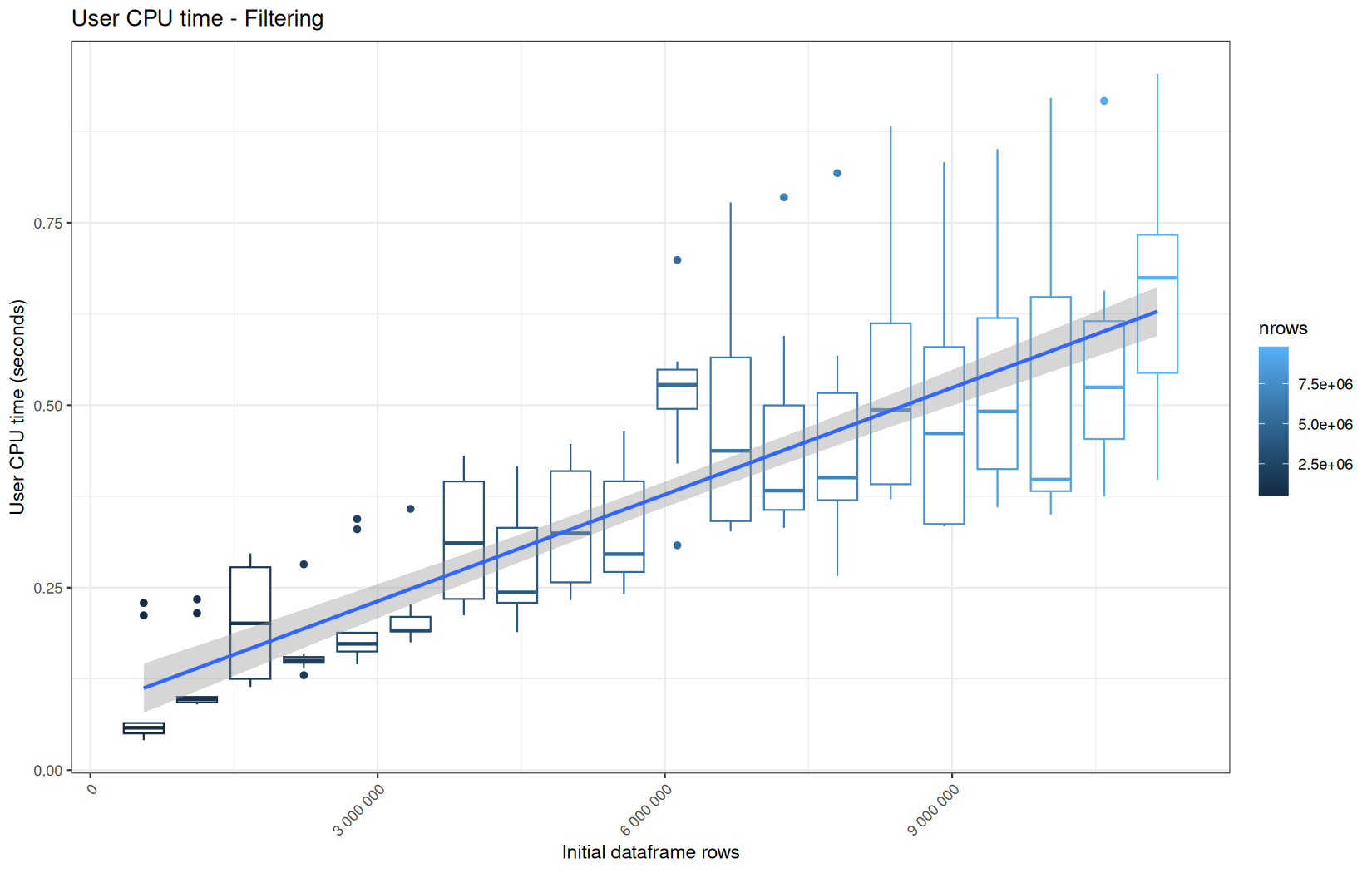
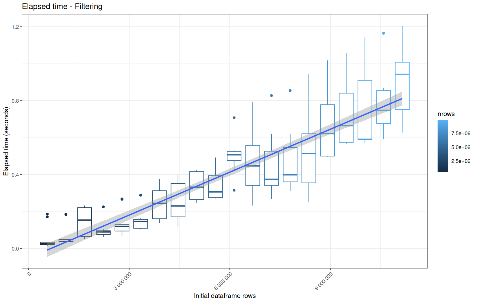
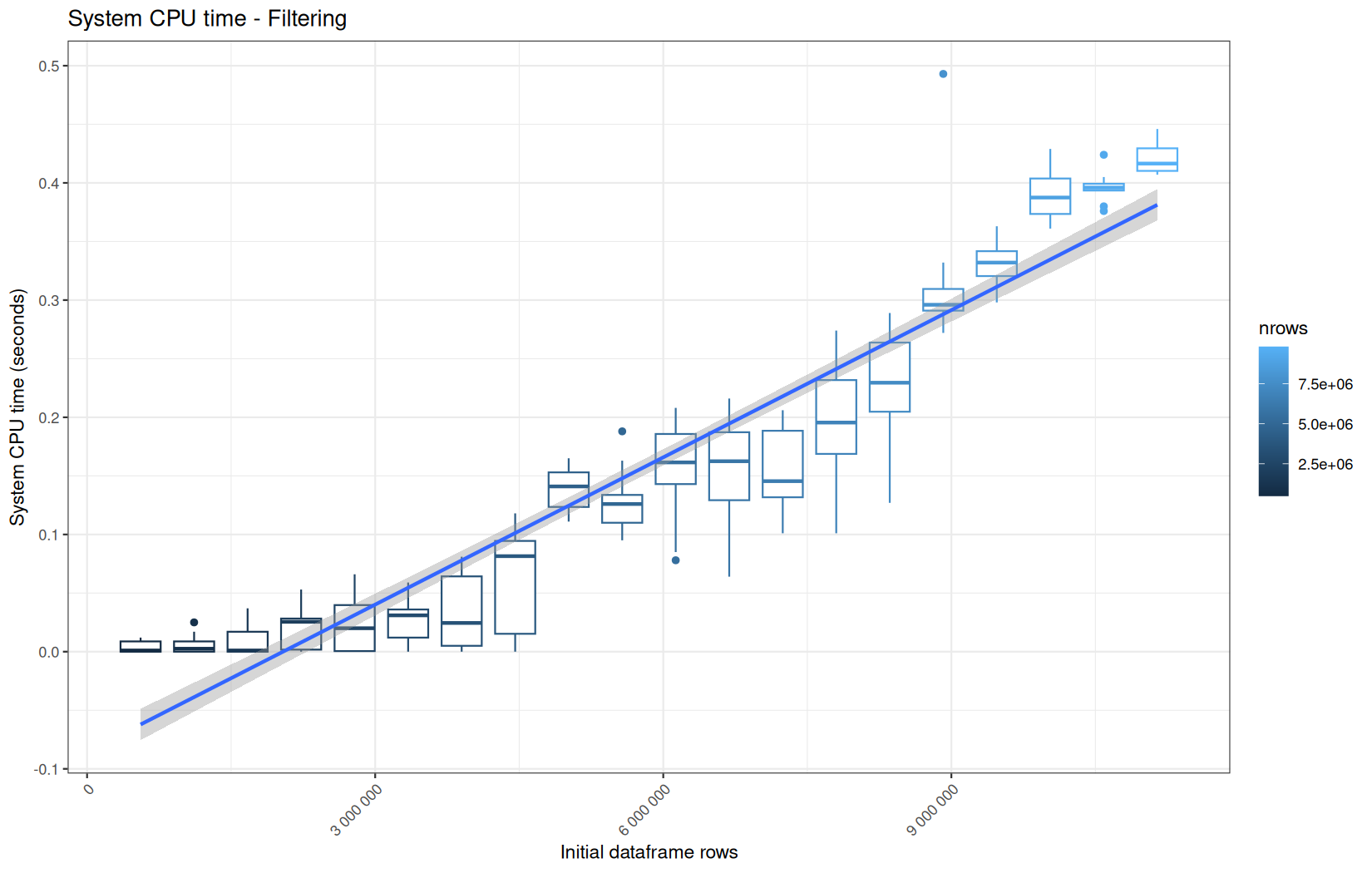
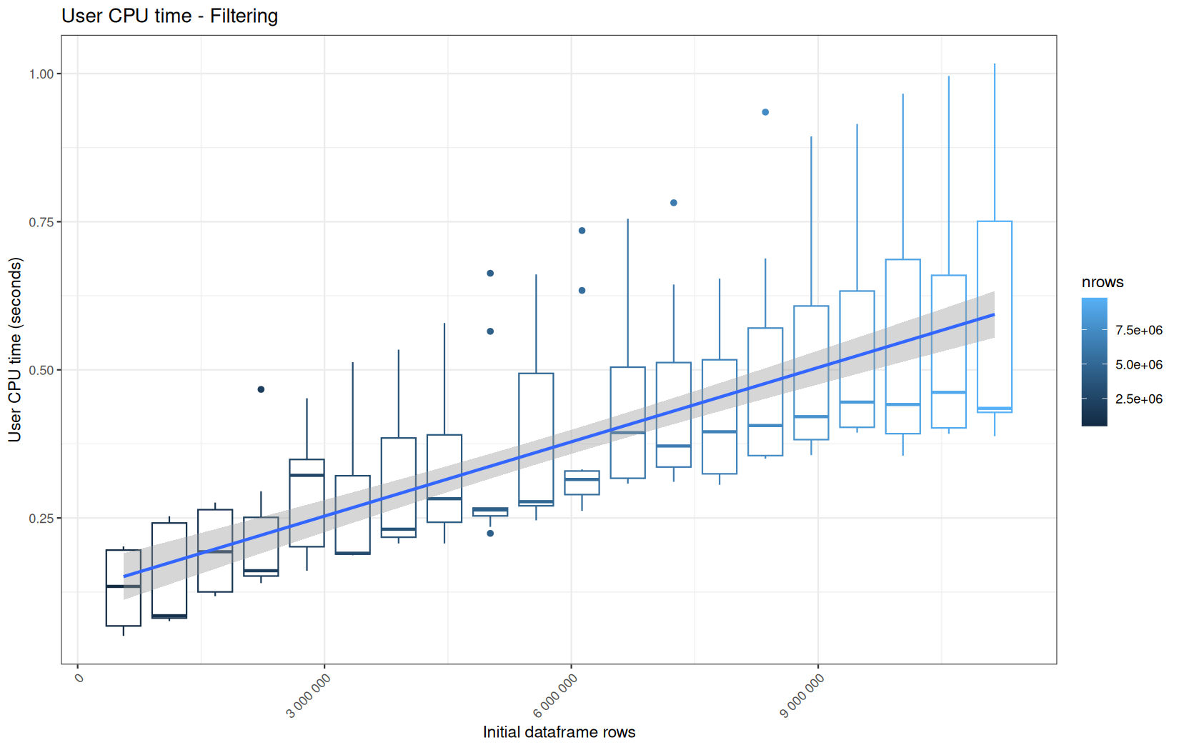
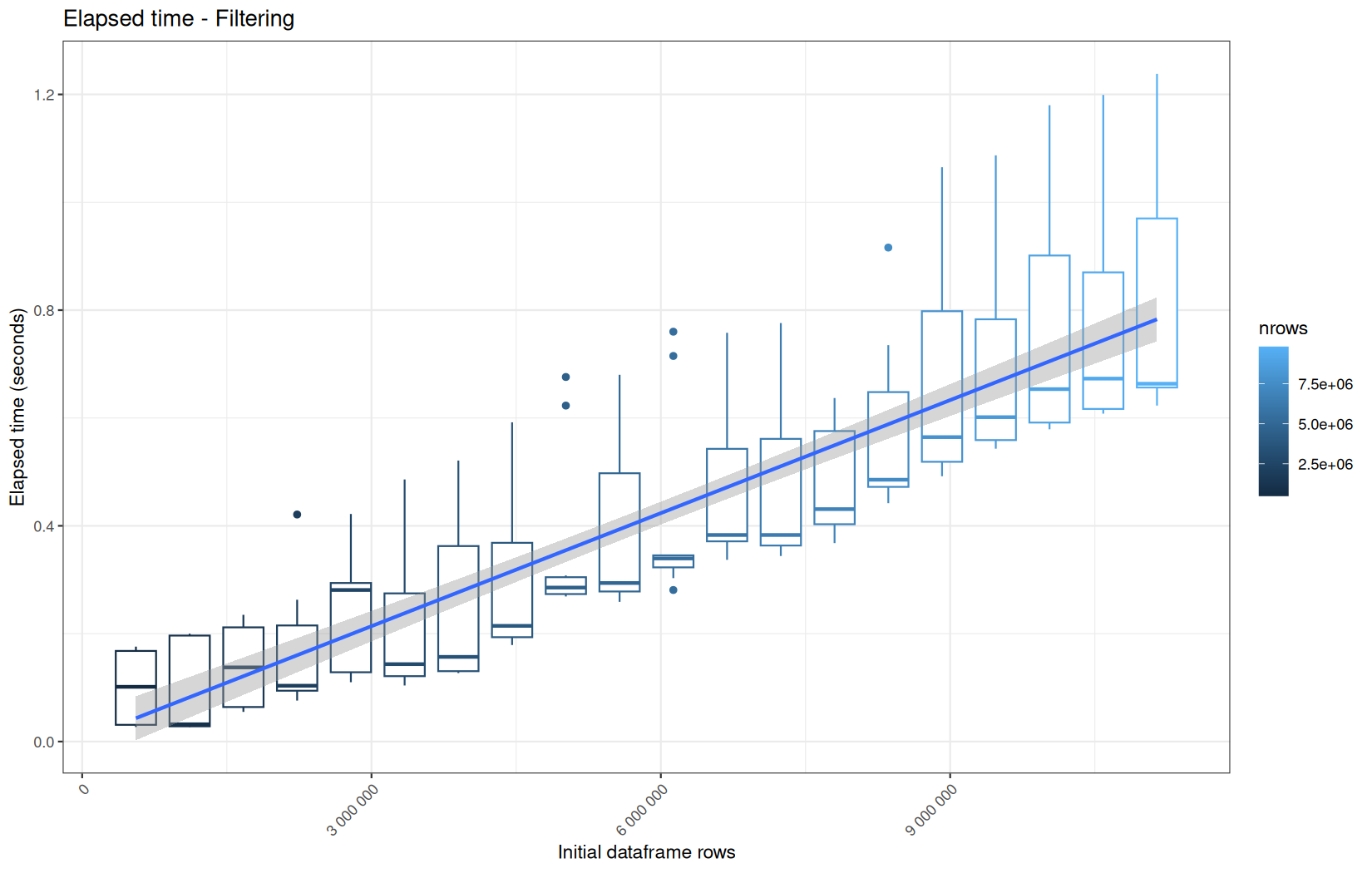
Roughly same profile.
dplyr
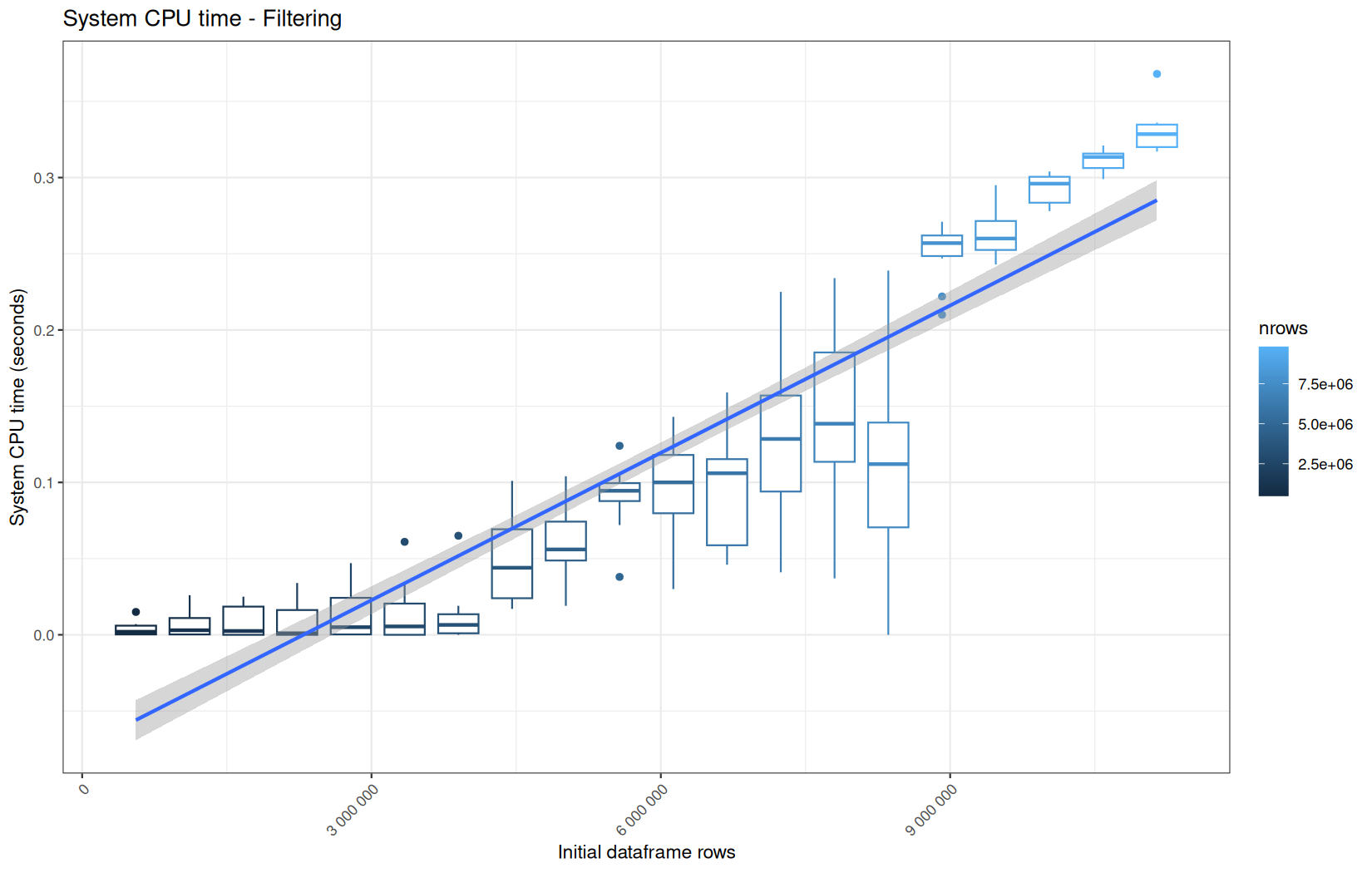
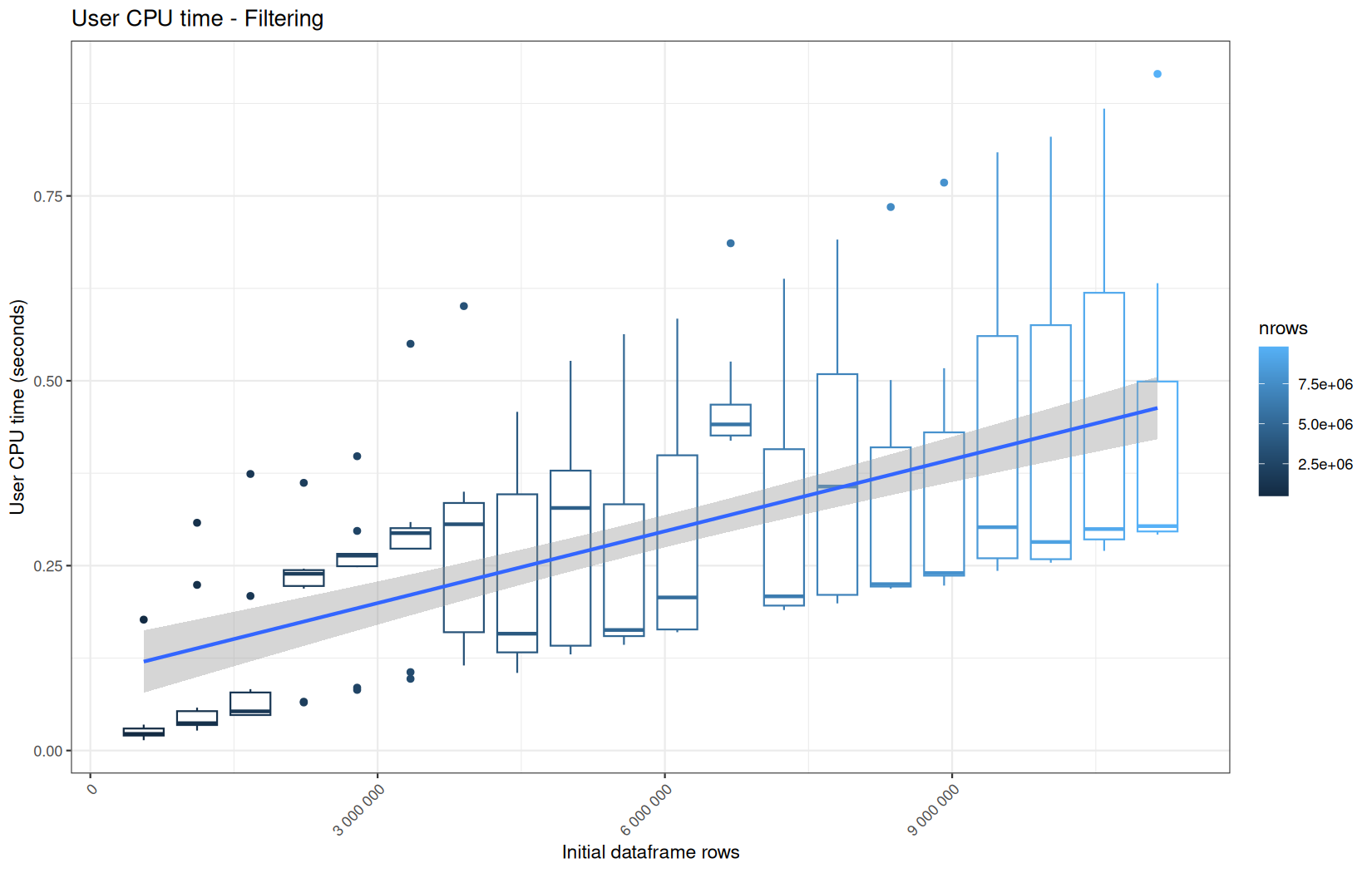
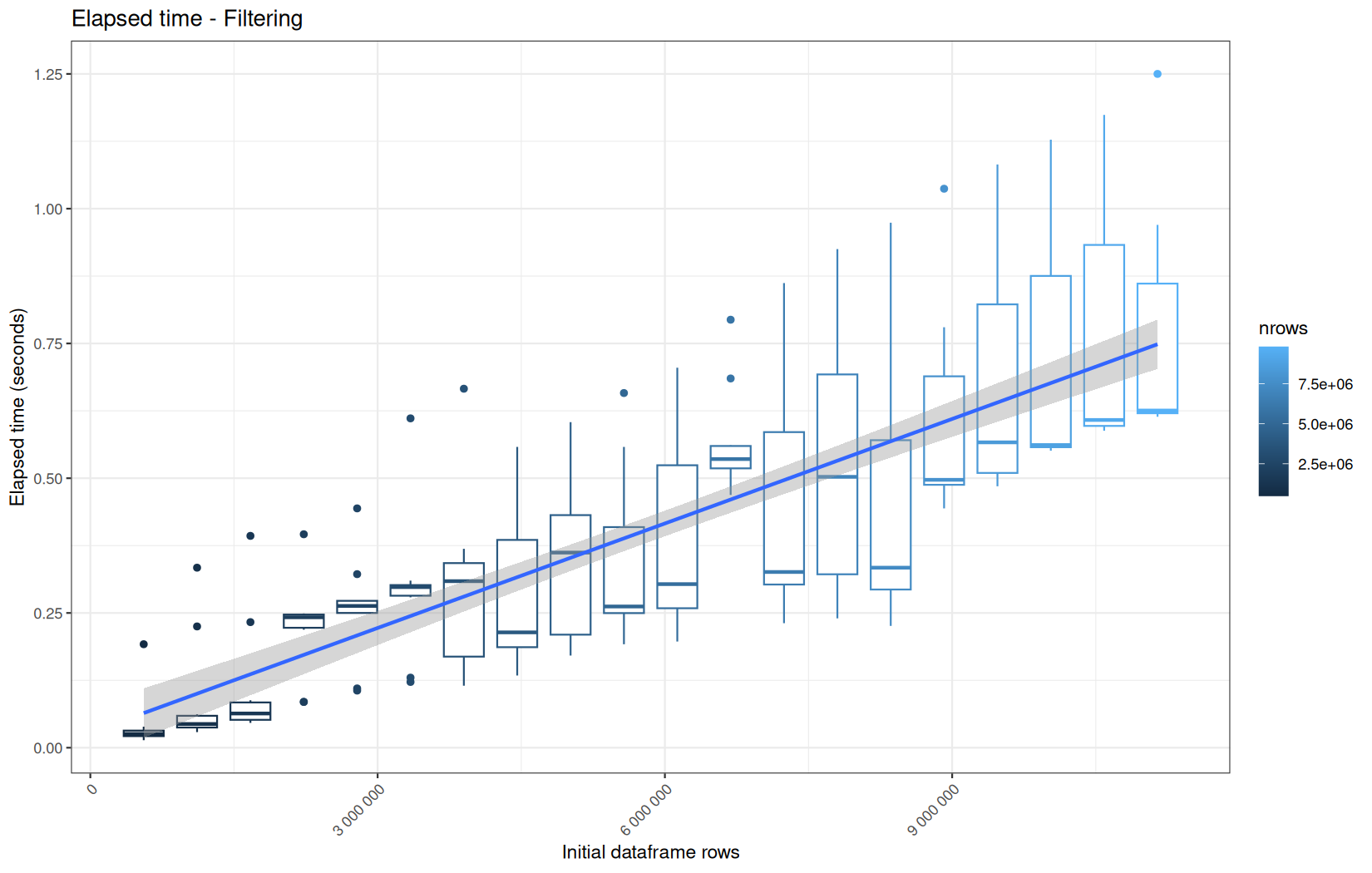
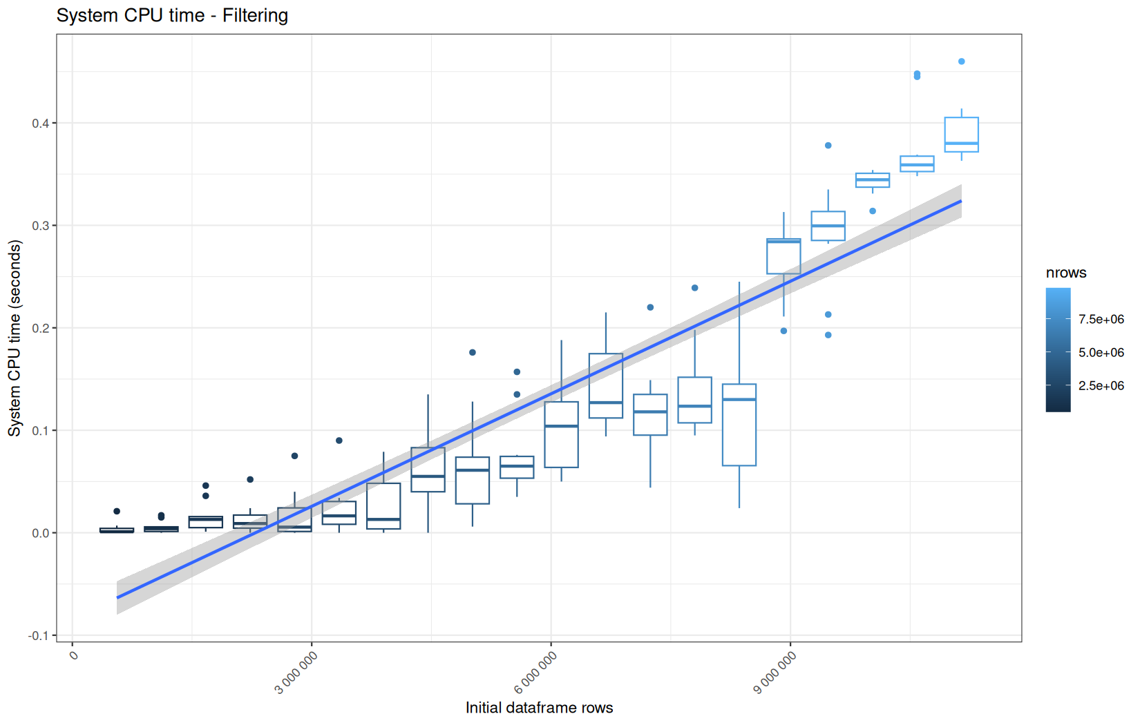
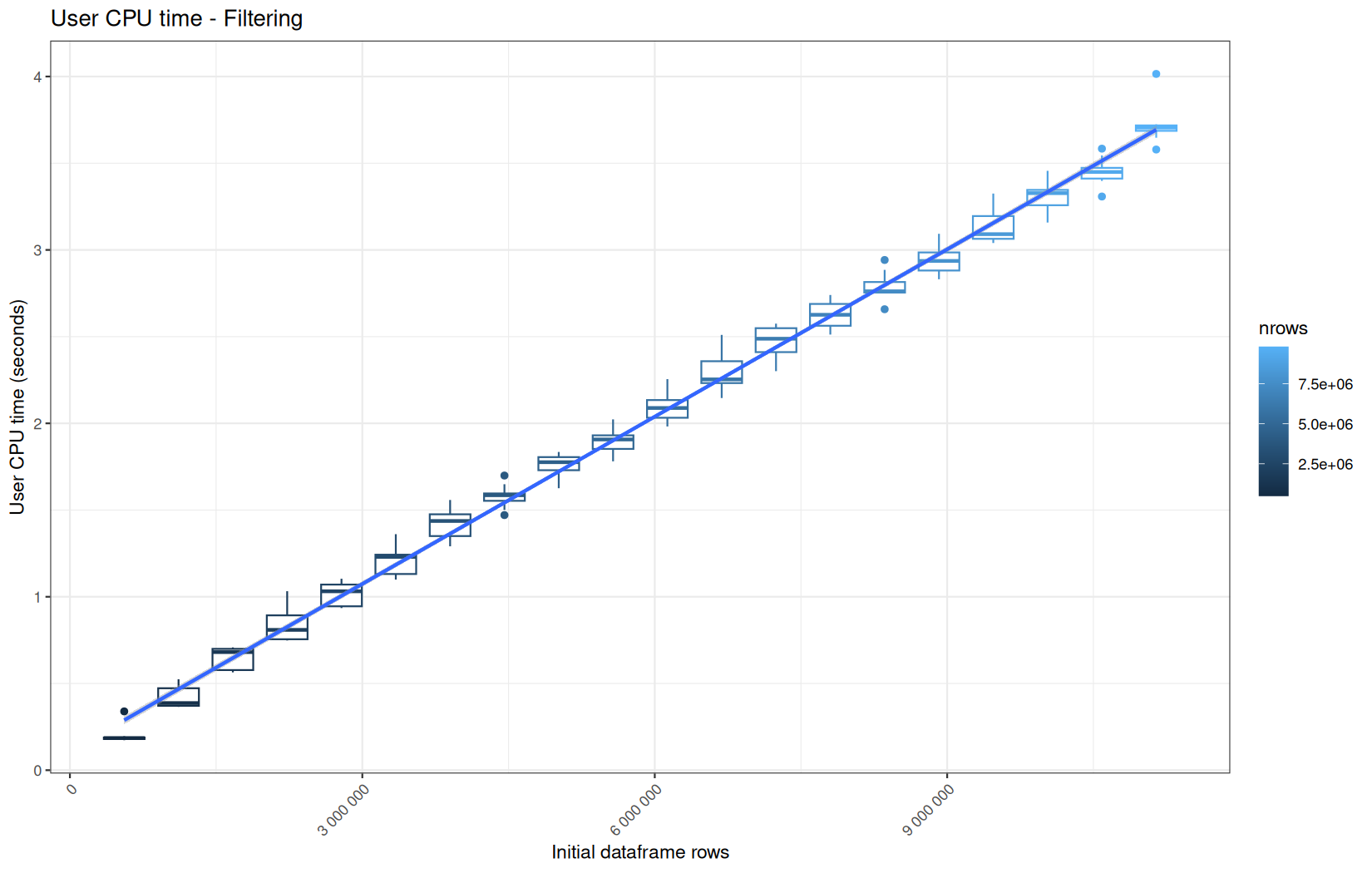
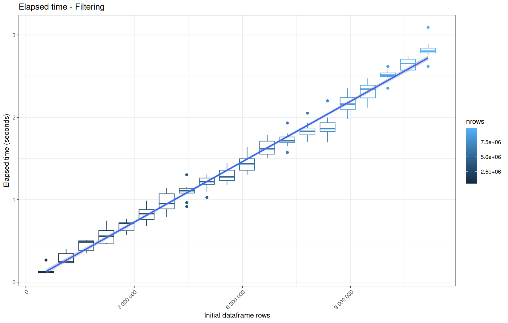
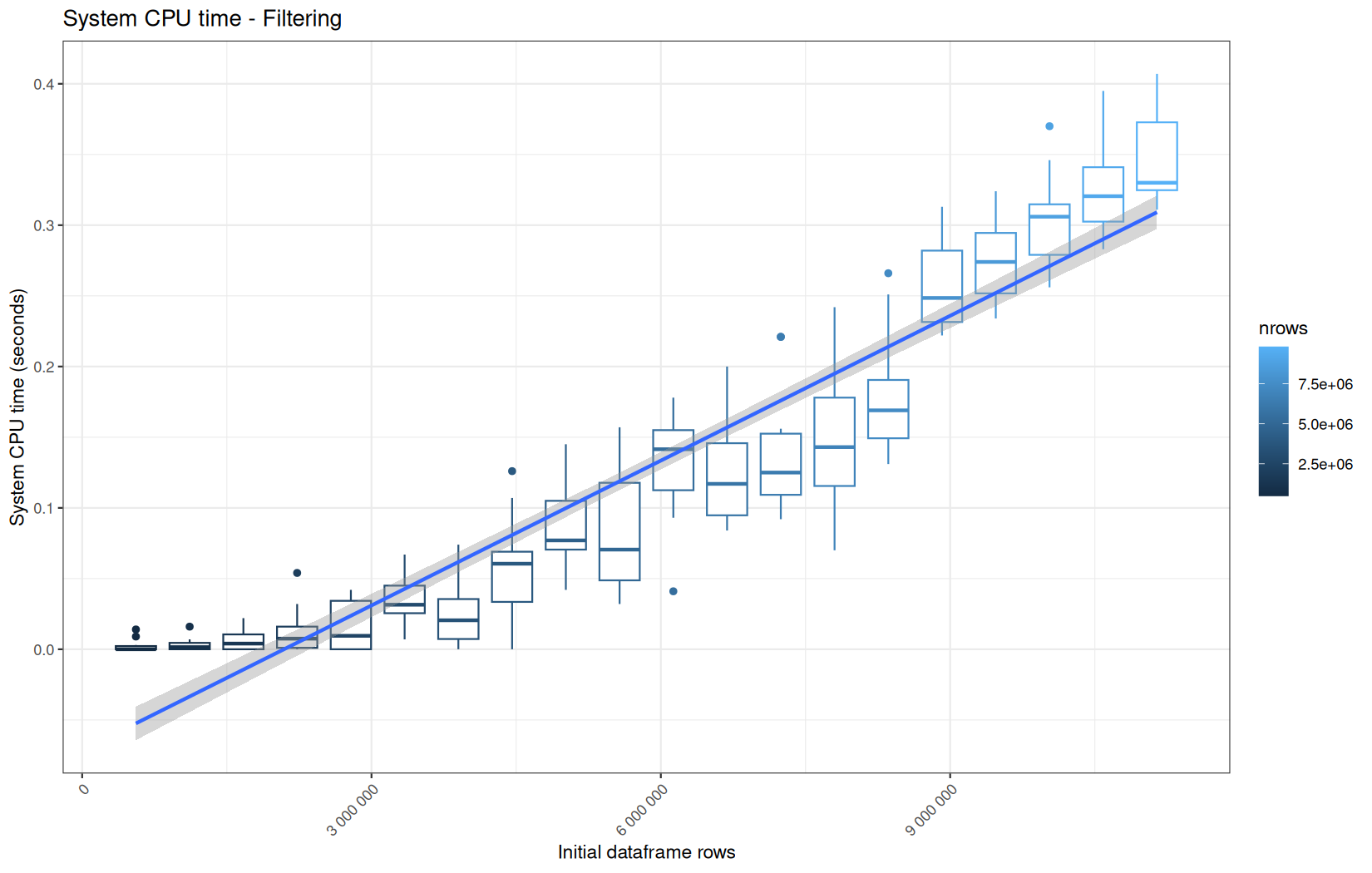
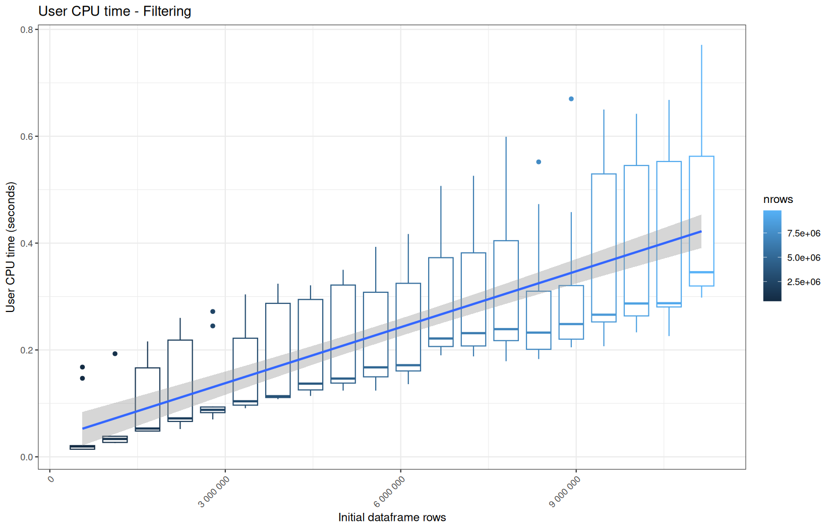
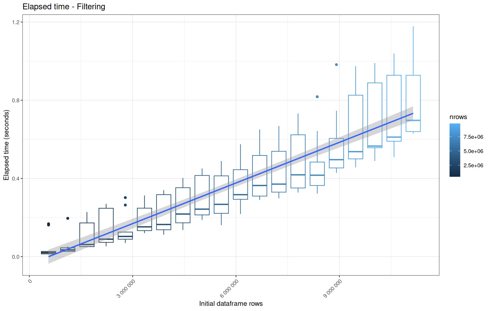
No surprise that the vroom + dplyr performs worst here, again due to delayed materialization, and this time on more than one column, here we see that target and status must be materialized.
Also, we clearly see that the materiaization is multithreaded here because the user time is higher than the elapsed time, maybe one thread for each column.
Data manipulation functions
We will now focus on a diverse set of operations to obtain a broader range of measurements. This allows us to group algorithmically similar steps together and describe the behavior of each pipeline without analyzing every operation independently. The goal is to focus on the operations that matter most and use them to characterize the overall profile of each pipeline.
Now go for:
last <- input$last_n * mult_map[[input$time_unit]] * bench_index
cutoff <- max(df$date) - last
df <- df[date >= cutoff]
So filter on an already materialized column.
You see that the filtered dataframe gets larger as the log-file gets larger due to the incrementation of bench_index over the runs.
Because at this pointthe column we are working on is mlready materialized, we can drop the ingestion engine results and focus purely on data.table VS dplyr execution time.
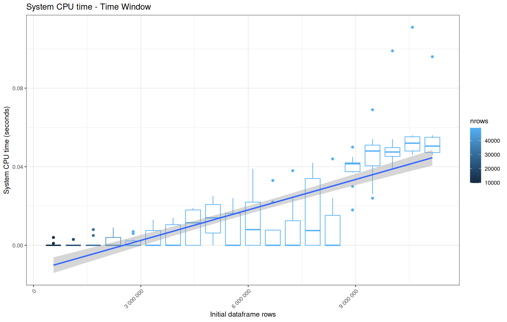
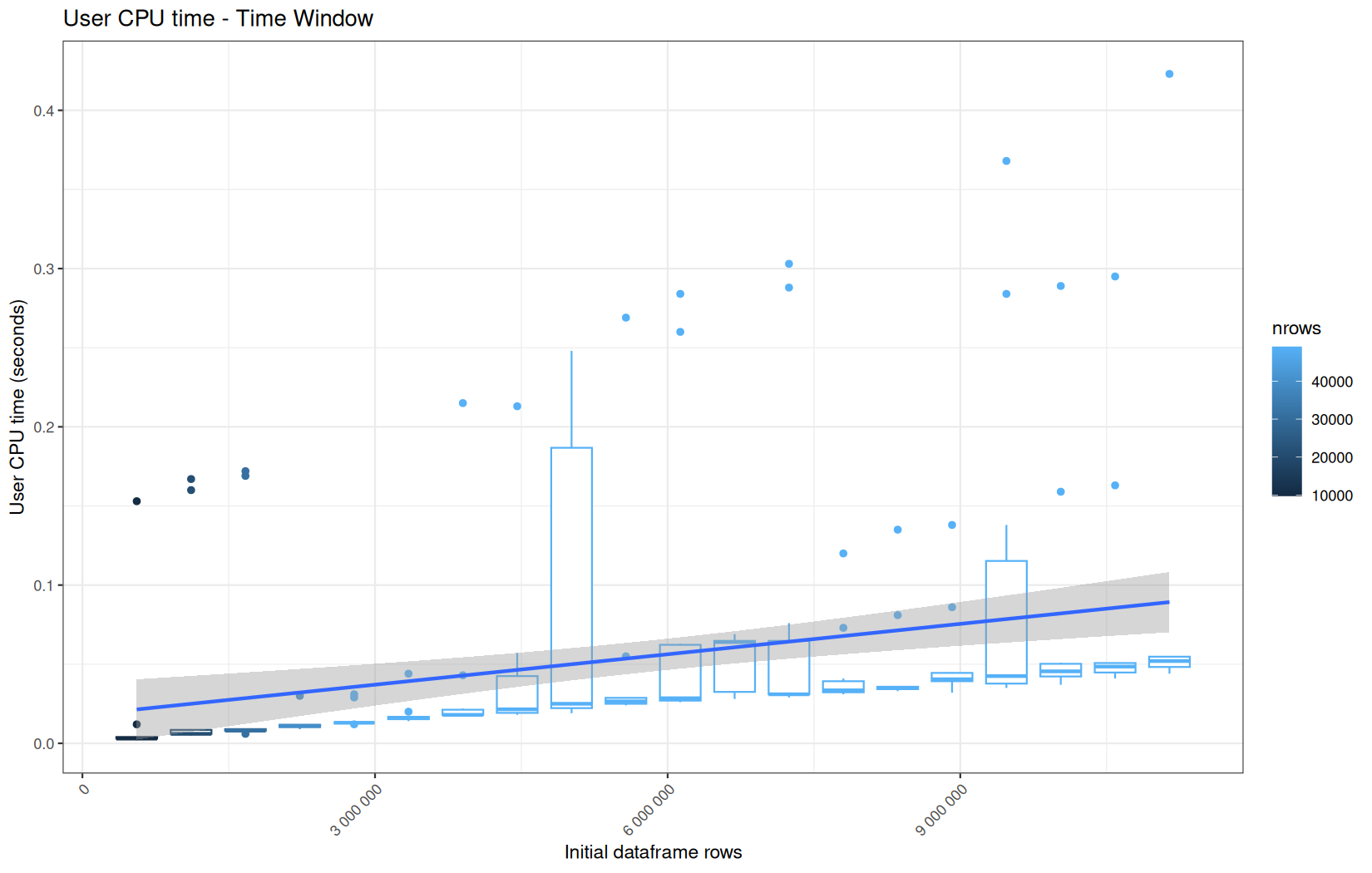
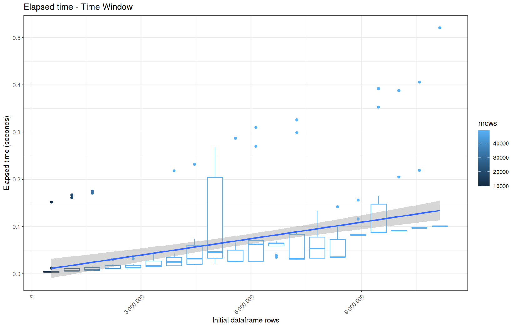
data.table
Same profile, but look at the cold-start.
Simple explanation in this operation, the sub-dataframe returned, or at least pârt of its vectors or columns can absolutely be cached for the later runs (mostly L2 or L3 at this point) because bench_index and max(df$date) does not change and are the only values where the sub-dataframe depends on.
dplyr
Ok, so it confirms the profile of the cold-start.
We can also note that the median of elapsed is arround 1 and was arround 0.5 for data.table.
This confirms what I measured in the previous article, data.table is often faster for filtering, even when the filter is semantically the same thing, i mean it is not an in-place operation.
The next operation that worth a benchmark is this one and its dplyr equivalent:
df[, sec := lubridate::floor_date(date, unit="second")]
df <- df[df[, .I[.N < 10], by = .(ip, sec)]$V1]
df[, sec := NULL]
Because it provides a group_by operation and we mostly spoke about filter.
It also drops a temp col.
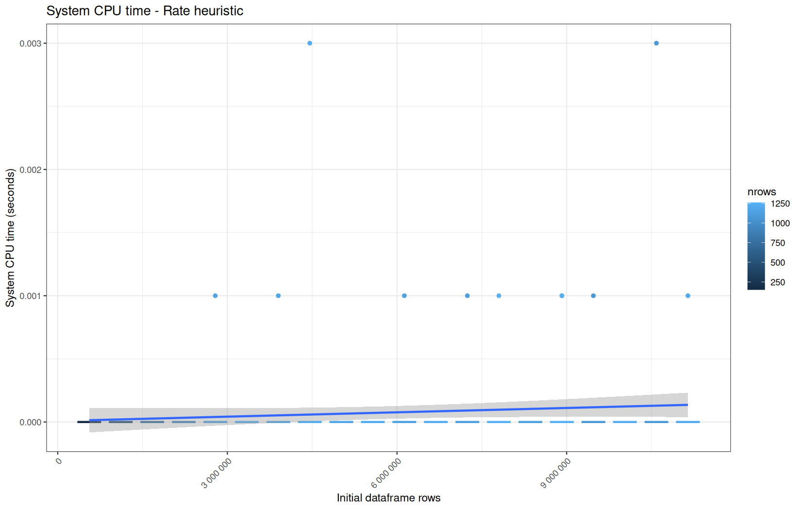
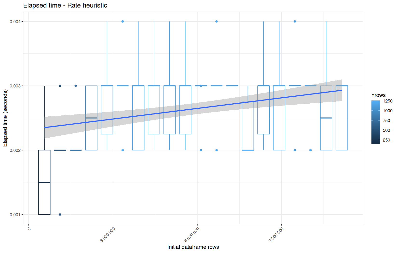
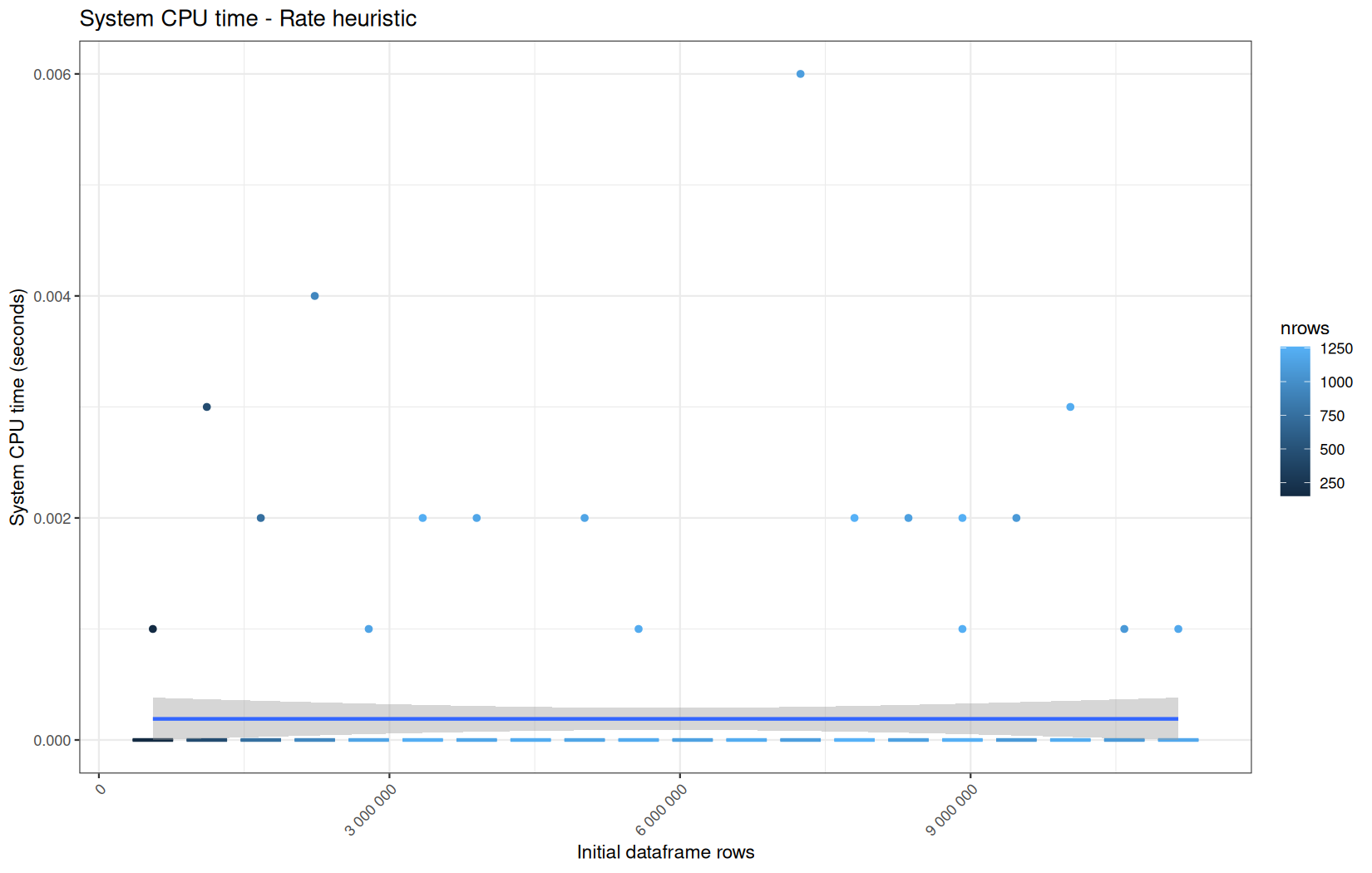
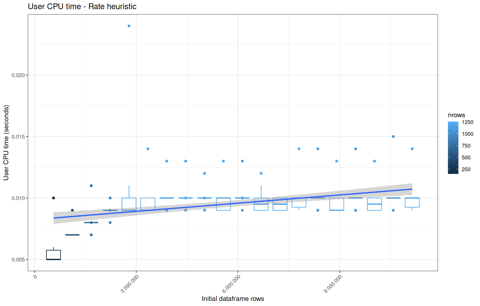
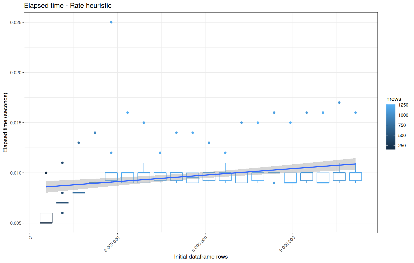
As yo see, contrary to the other operations the number of rows he operation is aplied on increase logarithmically.
That is a little annoying since we want the number of row to bee linearly increasing but we can nevertheless tell a story.
data.table
This is a very fast operation, the median of elapsed being in the miliseconds (below the dozen of ms).
We also see that this operation is multithreaded because user >> elapsed, but is that the group_by or the floor_date that is multithreaded ?
At this point we do not really know, so we will analyze the dplyr equivalent that also used floor_date from lubridate.
dplyr
Note, readr, dplyr and lubridate belongs to the tidyverse universe.
We see that elapsed is significantly higher than the data.table variant.
We also see that the operation is not multithreaded.
Because we also used floor_date here, we can infere that floor_date is also not mulithreaded and thatit was mostly the group_by operation in the data.table variant that was multithreaded.
Now there is a cool operation to benchmark that have column creation, column rearrangment, filtering and column drop.
data.table::setorder(df, ip, date)
df[, next_date := shift(date, type="lead"), by = ip]
df[, time_on_page := data.table::fcoalesce(
as.numeric(difftime(next_date, date, units = "secs")),
-1
)
]
keep <- df$time_on_page == -1 | (df$time_on_page > 5 & df$time_on_page < 3600)
df <- df[keep]
df[, next_date := NULL]
And its dplyr equivalent.
The new thing here is column creation with the per library intrisincs; coalesce.
This operation is special on the dplyr side, it is why we are just going to give one data.table path because all of their path are the same regardless of the ingestion engine.
But this is another story for the dplyr path -> the ingestion backend still had side-effect very visible here.
data.table
When it comes to the carinality, it is the same story as the previous operation.
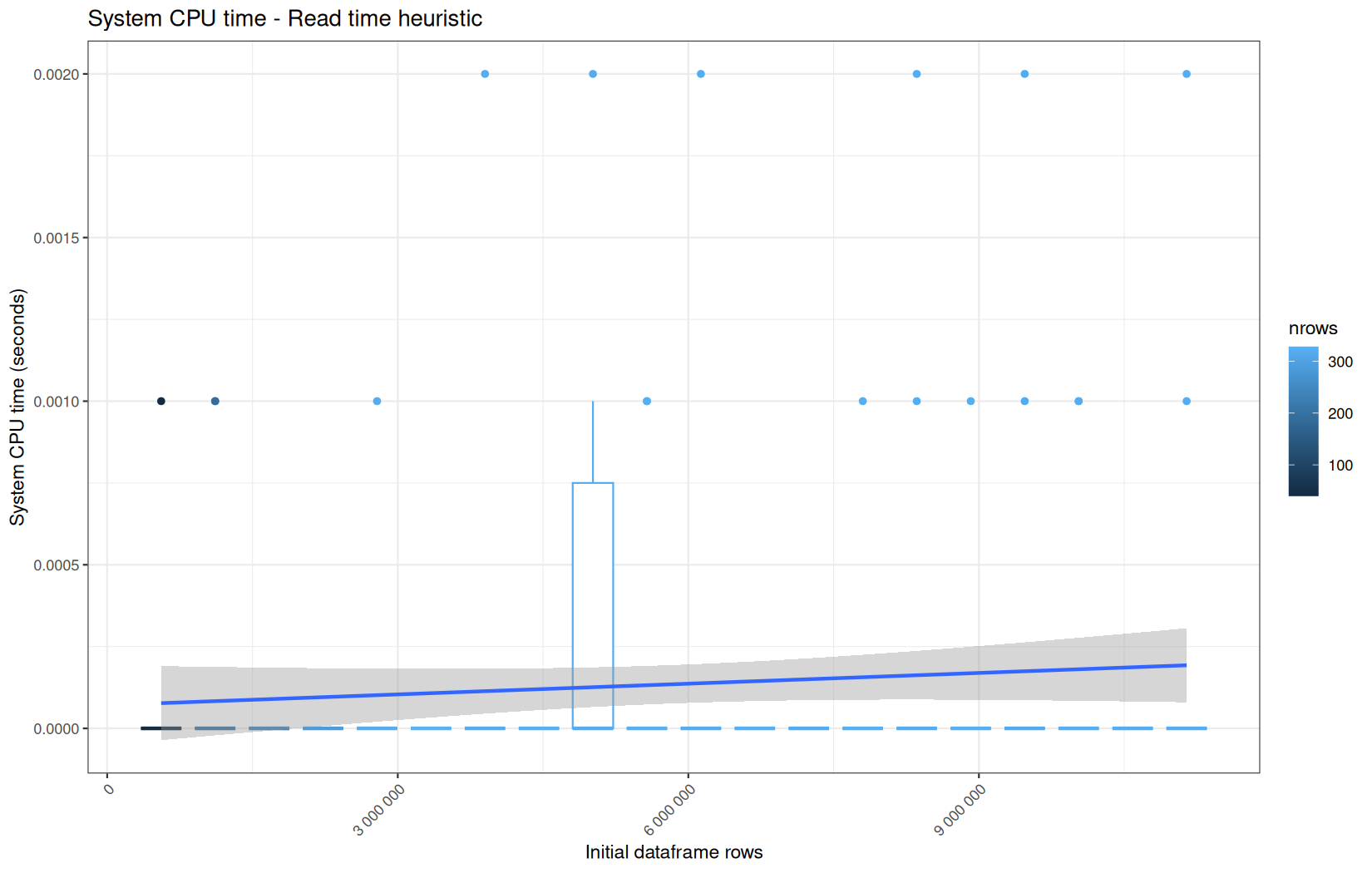
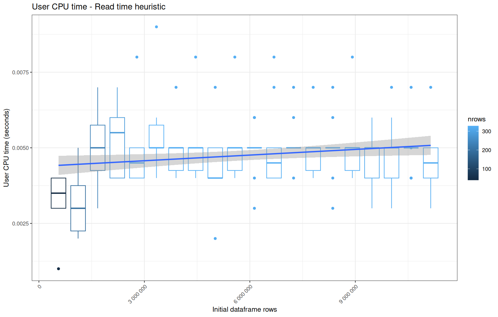
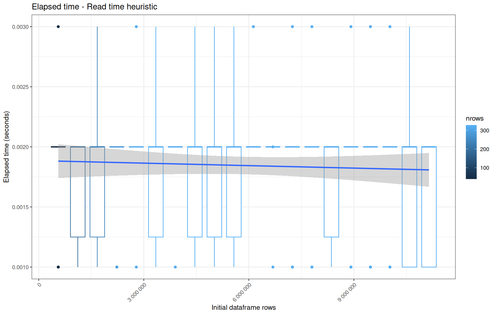
We can still say that the operation is multithreaded, because user >> elapsed.
The opertion that is multithreded is again the group_by ip here:
df[, next_date := shift(date, type="lead"), by = ip]
Another plausible contributor is data.table::setorder(). Unlike setcolorder(), which mostly rearranges column pointers, setorder() performs a real row sort. Here it orders the table by two keys: ip first, then date within each ip.
My intuition, as someone also working on dataframe internals, is that this kind of operation naturally exposes parallelism. Once the first key has partitioned, grouped, or otherwise organized the rows by ip, the second-key ordering by date can potentially be performed independently inside different ip groups or chunks of groups. In other words, the implementation does not necessarily have to treat the whole table as one indivisible sequential sort from beginning to end.
I am not claiming that this is exactly how data.table implements setorder() internally here, because this benchmark does not isolate that function. But algorithmically, a n-key row ordering operation is a credible candidate for the observed user > elapsed profile.
And the execution time is lower than the following dplyr variant as you'll see.
dplyr
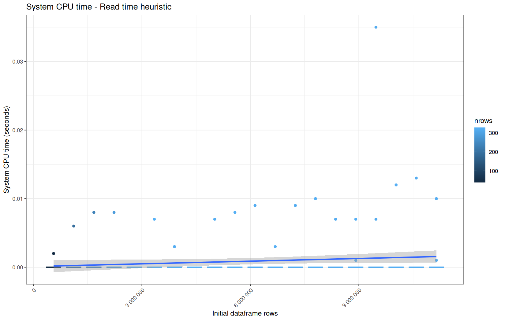
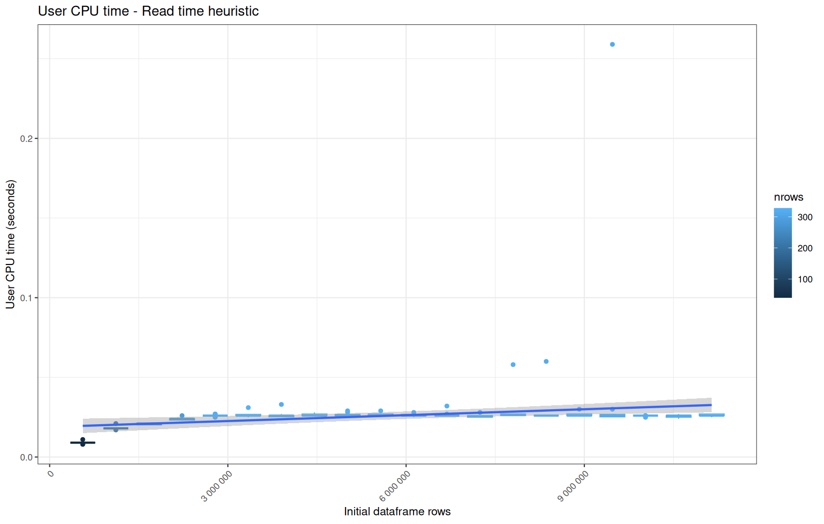
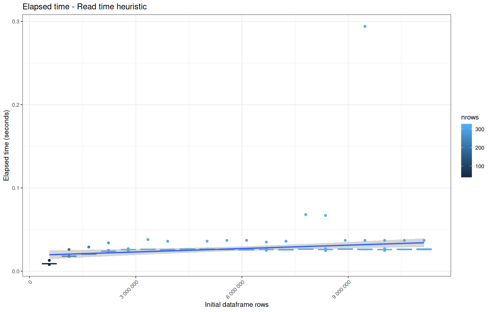
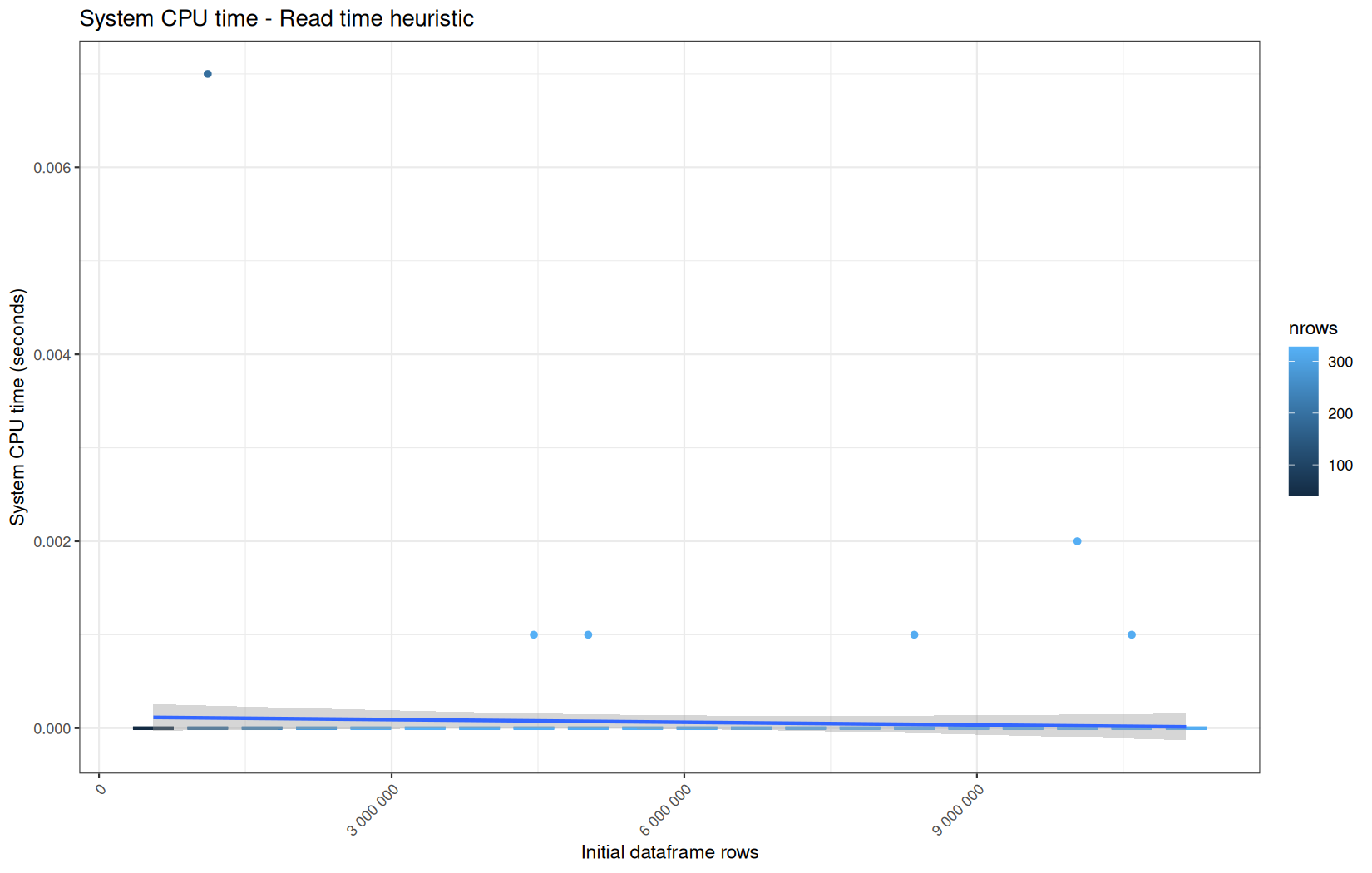
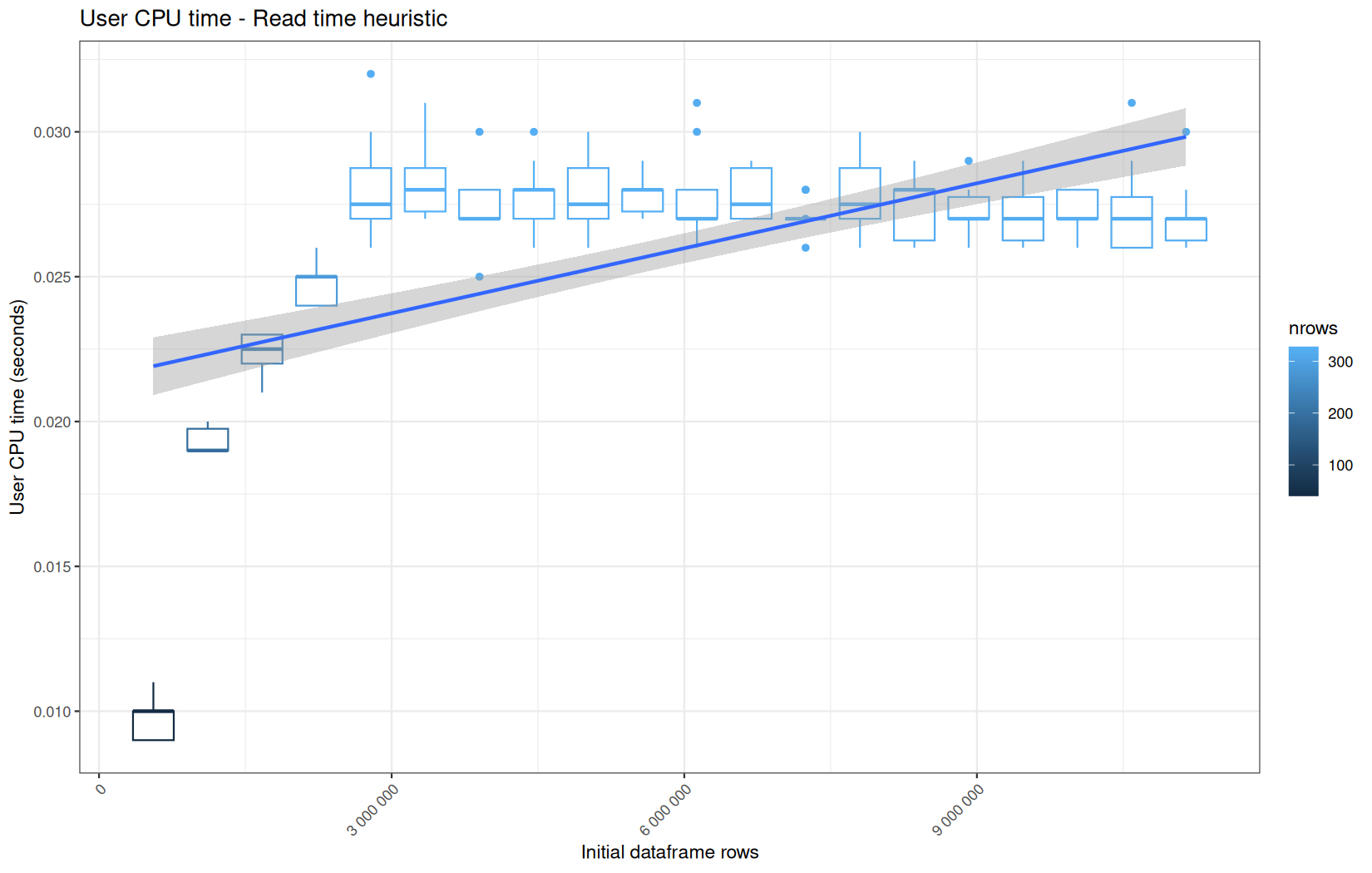

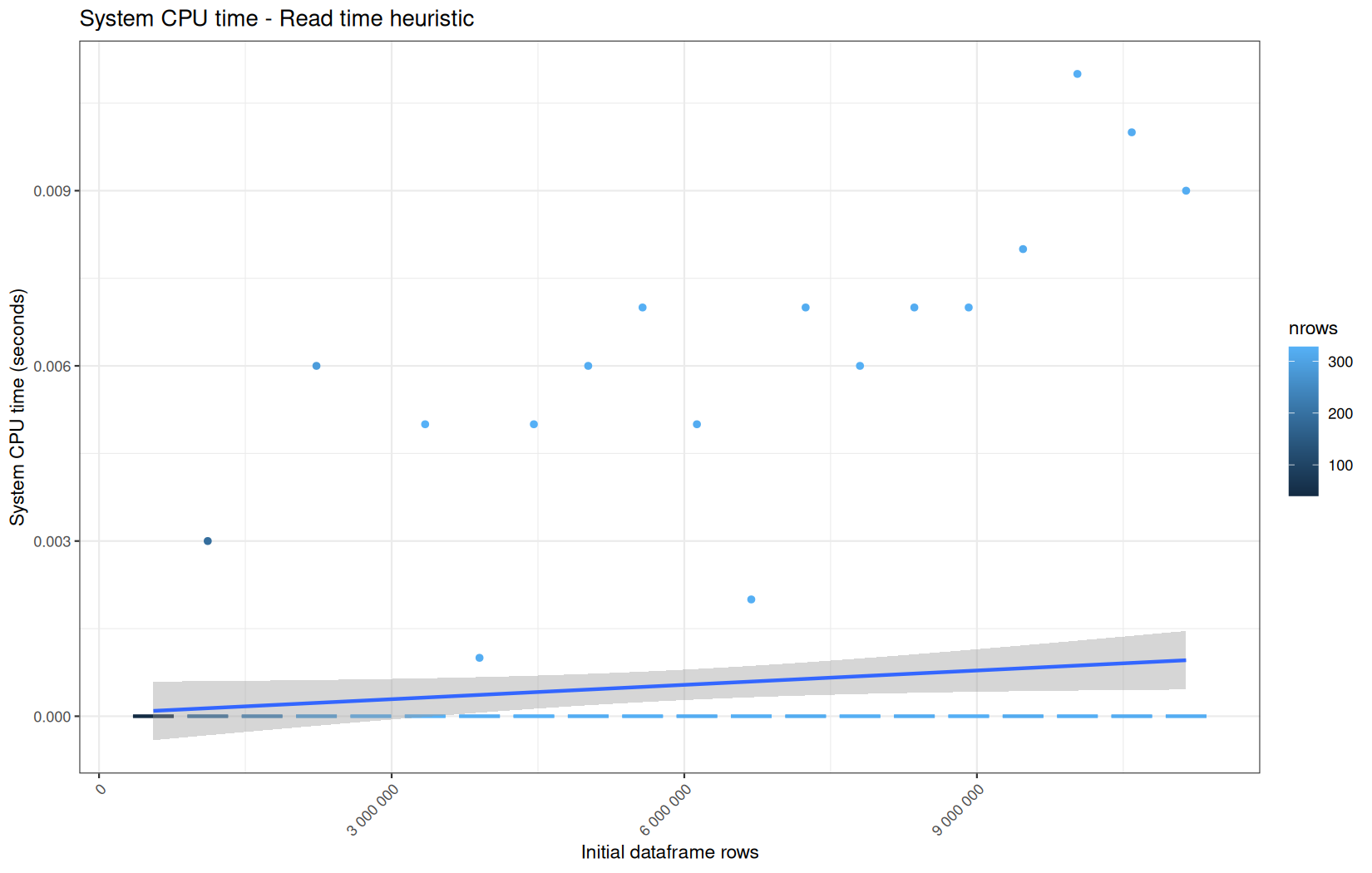
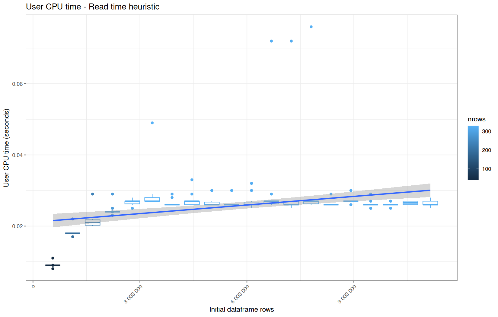
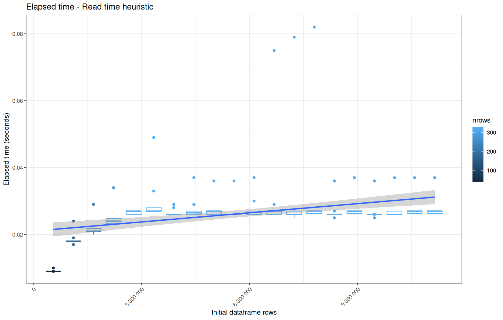
We see that the overall elapsed has the same profile everywhere here.
We work on arround 300 rows, so some profiles variantion can be explained by noise.
But we just note a huge cold-start outlier in the elapsed_time, user_time and system_time for readr path, but not concluding.
We also note thatfor the same path, its system_time is an order of magnitute higher than for the other path, but again I no algorithmic explanation for that.
Total
But all those individual graphs do not provide us a way to see in one picture the total behaviour of the pipeline per-metric across all the operations and especially compared to other configurations.
So, here are a per-operation and per-configuration metrics box-plots:
elapsed_time
  <button class="matrix-tab-row active" data-row="system">system</button>
  <button class="matrix-tab-row" data-row="user">user</button>
  <button class="matrix-tab-row" data-row="elapsed">elapsed</button>
</div>

<div class="matrix-tabs-row">
  <span class="matrix-tabs-label">Backend</span>

  <button class="matrix-tab-col active" data-col="readr">readr::read_tsv()</button>
  <button class="matrix-tab-col" data-col="vroom">vroom::vroom()</button>
  <button class="matrix-tab-col" data-col="fread">fread()</button>
</div>