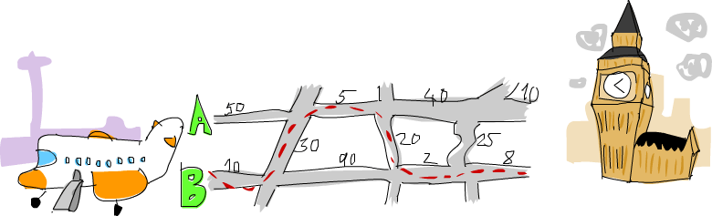
I will explain from my point of view the solution to the following problem https://learnyouahaskell.com/functionally-solving-problems#heathrow-to-london, we explore a recursive approach to solving an optimal path problem — where at each step, multiple paths are possible, and we must decide which route minimizes the total cost.

The idea is to think of the problem as a sequence of blocks — each representing a segment of possible movements. Between these blocks, we must choose how to transition optimally while keeping track of cumulative costs along each possible path.

1. The block model and mental picture

We can think of the system as three tracks: A, B, and C. Each block of the path has three values representing the cost of traveling along each of these tracks (or switching between them).

We define a small data type for the tracks:

data Track = A | B | C deriving (Show)

And a sample path consisting of four “blocks,” each represented by a triple of numeric costs:

myPath :: (Num a) => [(a, a, a)]
myPath = [
          (50, 30, 10), 
          (5, 20, 90), 
          (40, 25, 2),
          (10, 0, 8)]

Each tuple (a, c, b) can be seen as a block partition — a local cost structure that links the three tracks together. The challenge: for each step, we must choose whether to stay on the current track or switch to another one via the middle connection C.

2. The challenge: uncertainty and simultaneous tracking

One key insight is that we never know in advance which path will end up being optimal, because the cost of the next block may flip the decision. Therefore, we need to keep track of both potential optimal paths as we go forward.

This means we simultaneously carry:

• The sequence of tracks chosen for path 1 (xs1)
• The sequence of tracks chosen for path 2 (xs2)
• The cumulative sums (sum1 and sum2) for each path

At every step, we compare local costs and decide which way to extend each path — without discarding either until the very end.

3. The recursive optimal path function

The function optimalPath carries all of this information through recursion:

optimalPath :: (Num a, Ord a) => ([(a, a, a)], [Track], [Track], a, a) -> ([Track], a)
optimalPath ([], xs1, xs2, sum1, sum2)
    | sum1 < sum2 = (reverse xs1, sum1)
    | otherwise = (reverse xs2, sum2)
optimalPath ((a, c, b):xs, xs1, xs2, sum1, sum2) 
    | b + c > a = if a + c > b
                  then optimalPath (xs, A:xs1, B:xs2, sum1 + a, sum2 + b)
                  else optimalPath (xs, A:xs1, C:A:xs1, sum1 + a, sum1 + a + c)
    | otherwise = if a + c > b
                  then optimalPath (xs, C:B:xs2, B:xs2, sum2 + b + c, sum2 + b)
                  else optimalPath (xs, C:B:xs2, C:A:xs1, sum2 + b + c, sum1 + a + c)

Let’s break it down:

• If there are no more blocks left ([]), the recursion ends. We simply compare sum1 and sum2 and return the smaller one — the best path overall.
• Otherwise, we look at the current block (a, c, b) and the costs of each connection.
• We update both potential paths based on which local transitions are more optimal, propagating both cumulative costs recursively.

4. The mental model of the algorithm

Imagine you are walking down two possible corridors, A and B, connected at certain points by a bridge C. At every step, you can:

• Continue along your current corridor
• Cross the bridge to switch corridors (paying an extra cost c)

The problem is that you never know if switching will pay off later — maybe the next segment will make the other corridor much cheaper. So, instead of guessing, you keep both paths alive at each recursion step. This is the core intuition of the algorithm.

By the time you reach the last block, you simply compare the accumulated sums and pick the better one.

5. A concrete example

Let’s run it on myPath:

main = print (optimalPath (myPath, [], [], 0, 0))

The output will show:

• The optimal sequence of tracks to take
• The total minimum cost

The structure of recursion ensures that, regardless of the number of blocks, the algorithm will always track both possible optimal paths and converge on the best one at the end.

6. What this teaches about recursive design

This project demonstrates an important principle in Haskell (and functional thinking in general):

• When the future is uncertain, carry forward all possible states and decide later.
• Recursion naturally models step-by-step reasoning across a sequence of decisions.
• By building immutable state updates (paths and sums), the code remains pure, transparent, and easy to test.

7. Wrap-up

The “optimal path” algorithm is more than a cost minimization trick — it’s an example of recursive dynamic reasoning in a purely functional language.

At each block:

• We compare local transitions (a, b, and c).
• We maintain both evolving path states (xs1 and xs2).
• We move forward, trusting recursion to accumulate and finalize the decision.

This approach — maintaining all viable states until the end — captures the essence of functional problem solving: describe the process, not the mutation.

And with just a few lines of Haskell, we model a decision system that stays both elegant and robust.